By Sagi Shaier · 31 October 2026 · 9 min read
Word2Vec explained: skip-gram vs CBOW
How a small prediction task produces word vectors, what separates the skip-gram and CBOW versions, and how to write both in PyTorch with real output at each step.
Word2Vec is a method for learning a short list of numbers for each word by training a small model to guess which words appear near each other. Words used in similar places end up with similar numbers, so a program can measure how close two words are in meaning. It comes in two versions, skip-gram and CBOW, and they differ in which word the model has to guess.
What problem does Word2Vec solve?
A model needs words as numbers. An older route is to count: build a table with one row and one column per word, then record how often each pair of words appears close together. The table holds useful signal, because words with similar meanings tend to appear near the same words. It is also large and mostly zeros. With 50,000 words, every row holds 50,000 numbers, so the table usually needs compressing before it is practical.
Word2Vec keeps the same signal and skips the counting table. It trains a small neural network on a prediction task, where the input is one or more words and the target is a nearby word. The network holds an embedding table with one row of numbers per word. Training updates those rows over and over so the predictions improve. When training ends, the prediction task is thrown away and the rows are kept as the word embeddings.
What is a context window?
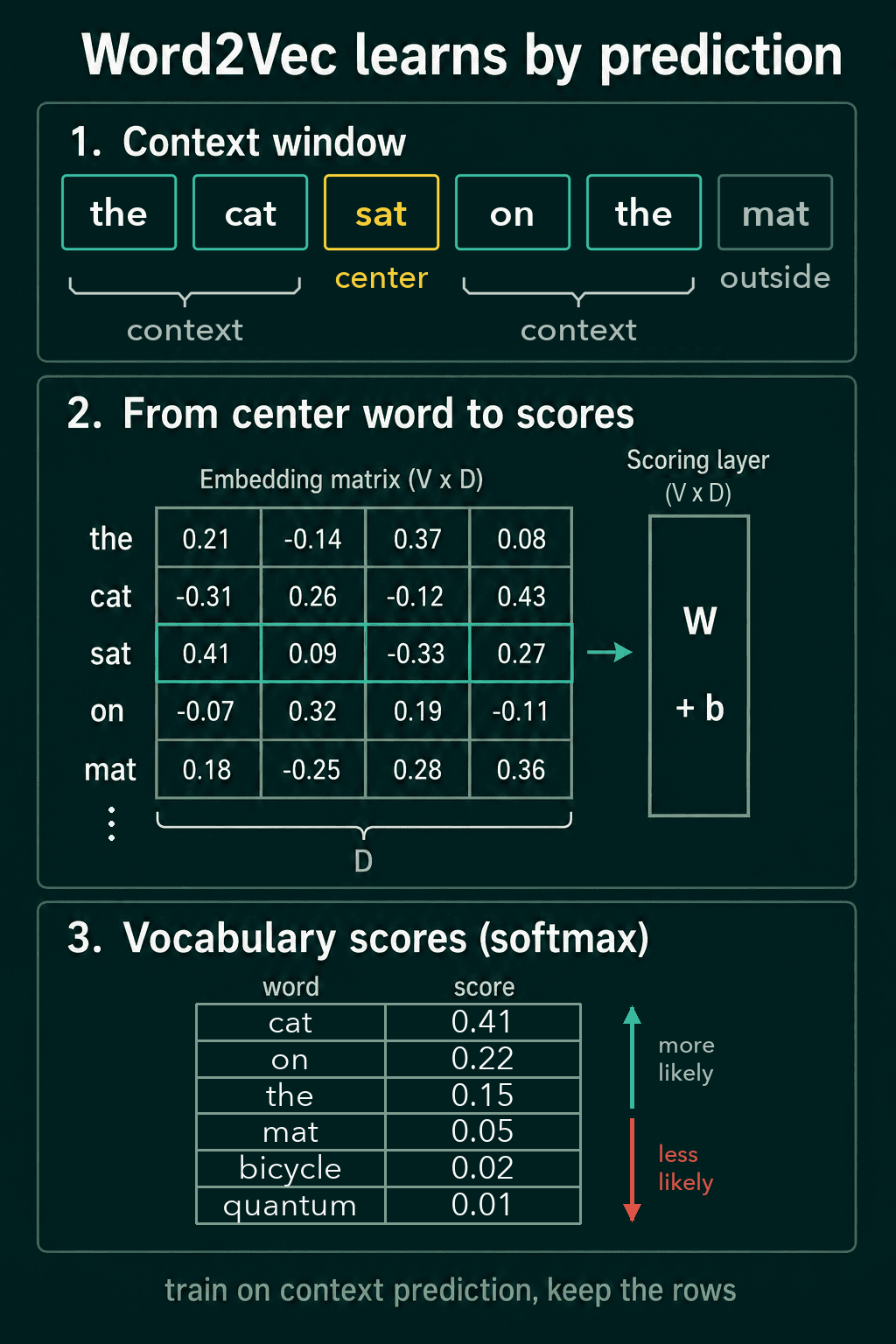
Both versions read text through a context window, which is a center word plus the $c$ words on each side of it. Take the sentence "the cat sat on the mat" with "sat" as the center and $c = 2$. The context words are "the" and "cat" on the left and "on" and "the" on the right. The word "mat" sits three positions away, so it is outside this window. The window then moves one word along and the next word becomes the center.
What is inside the network?
The network has two layers. Write $V$ for the number of words in the vocabulary and $D$ for the length of each word's row.
The first layer is the embedding table, which is a matrix with $V$ rows and $D$ columns. Giving it a word returns that word's row.
The second layer is a linear scoring layer. It multiplies that row by a weight matrix $W$, also $V$ by $D$, and adds a bias vector $b$. The result is $V$ numbers with one score per vocabulary word. A function called softmax then turns those scores into probabilities that add up to 1.
Skip-gram: predict the context from the center word
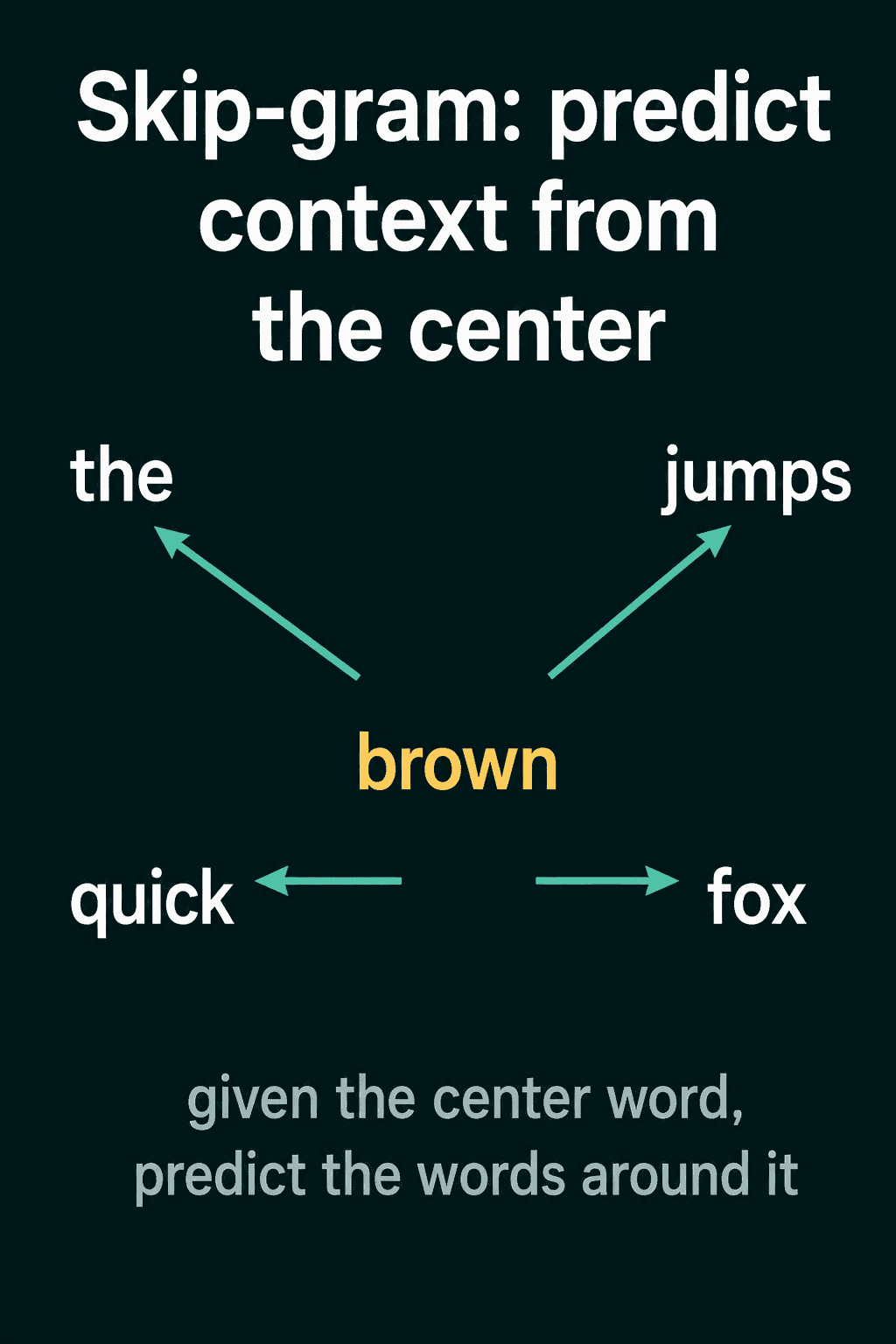
Skip-gram takes the center word and predicts the words around it. Take "the quick brown fox jumps over the lazy dog" with a window of 2. The center word "brown" predicts "the", "quick", "fox" and "jumps".
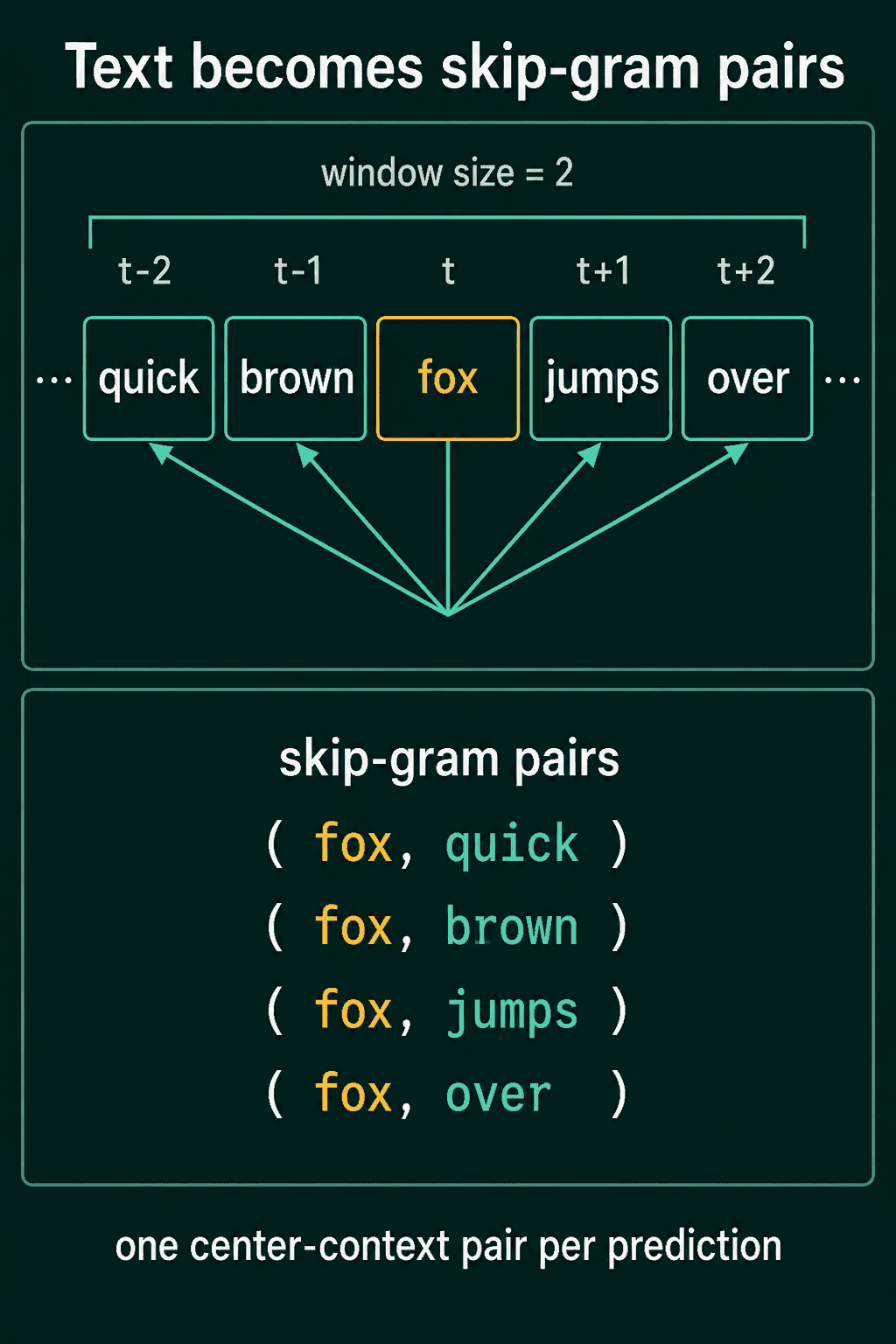
Each center word paired with one context word is a separate training example. So (fox, quick) and (fox, brown) are two different pairs. This function builds all of them:
1def get_skipgram_pairs(tokens, window_size):
2    pairs = []
3    for i, center in enumerate(tokens):
4        for j in range(i - window_size, i + window_size + 1):
5            if j < 0 or j >= len(tokens) or j == i:
6                continue
7            pairs.append((center, tokens[j]))
8    return pairs
9
10tokens = "the quick brown fox jumps over the lazy dog".split()
11pairs = get_skipgram_pairs(tokens, window_size=2)
12print(len(pairs))
13print(pairs[:5])
14print([pair for pair in pairs if pair[0] == "fox"])
It prints:
130
2[('the', 'quick'), ('the', 'brown'), ('quick', 'the'), ('quick', 'brown'), ('quick', 'fox')]
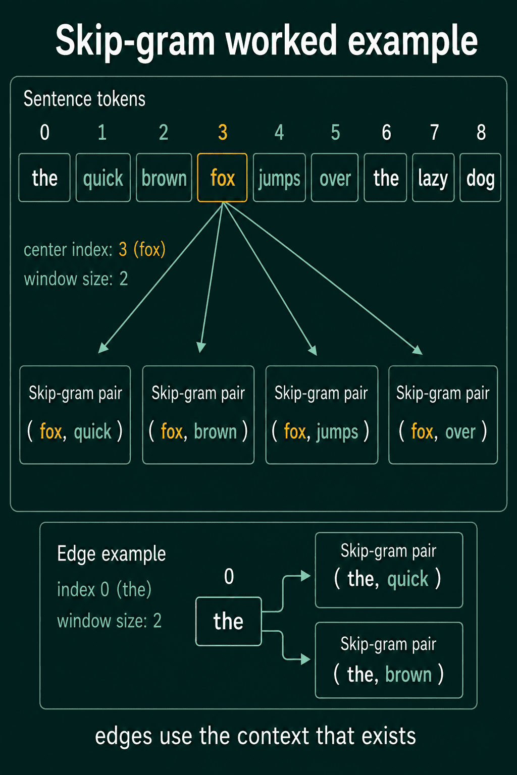
3[('fox', 'quick'), ('fox', 'brown'), ('fox', 'jumps'), ('fox', 'over')]
For each position i, the inner loop walks every position j from two words before to two words after. It skips j when it falls off either end of the list or lands on the center word.
The first word shows why the edge check is there. "the" at position 0 has nothing to its left, so it only gets two pairs, while "fox" at position 3 has a full window and gets four.
How skip-gram scores one pair
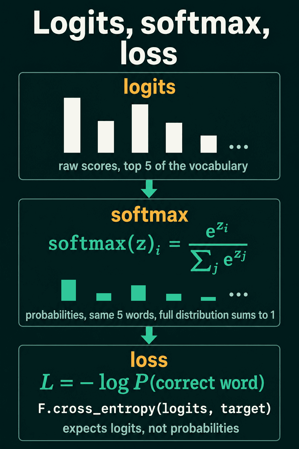
The scoring layer gives one raw score per vocabulary word. These raw scores are called logits, and they can be any real numbers, so they are not probabilities yet.
Softmax turns logits $z$ into probabilities. It raises $e$ to each score, then divides by the sum of all those values:
$$\text{softmax}(z)_i = \frac{\exp(z_i)}{\sum_j \exp(z_j)}$$
For example, say three words have logits 2.0, 1.0 and 0.1. Softmax gives 0.659, 0.242 and 0.099. The biggest logit gets the biggest probability and the three add up to 1.
The loss for one pair is the negative log of the probability given to the correct word:
$$L = -\log P(\text{correct word})$$
If the first word is the correct one, the loss is $-\log 0.659 = 0.417$. PyTorch computes the same number from the logits directly:
1import torch
2import torch.nn.functional as F
3
4logits = torch.tensor([2.0, 1.0, 0.1])
5target = torch.tensor(0)
6
7probs = F.softmax(logits, dim=0)
8print(probs)
9print(-torch.log(probs[target]))
10print(F.cross_entropy(logits, target))
It prints:
1tensor([0.6590, 0.2424, 0.0986])
2tensor(0.4170)
3tensor(0.4170)
F.cross_entropy expects logits and applies the softmax step itself, which is why the model code passes it raw scores.
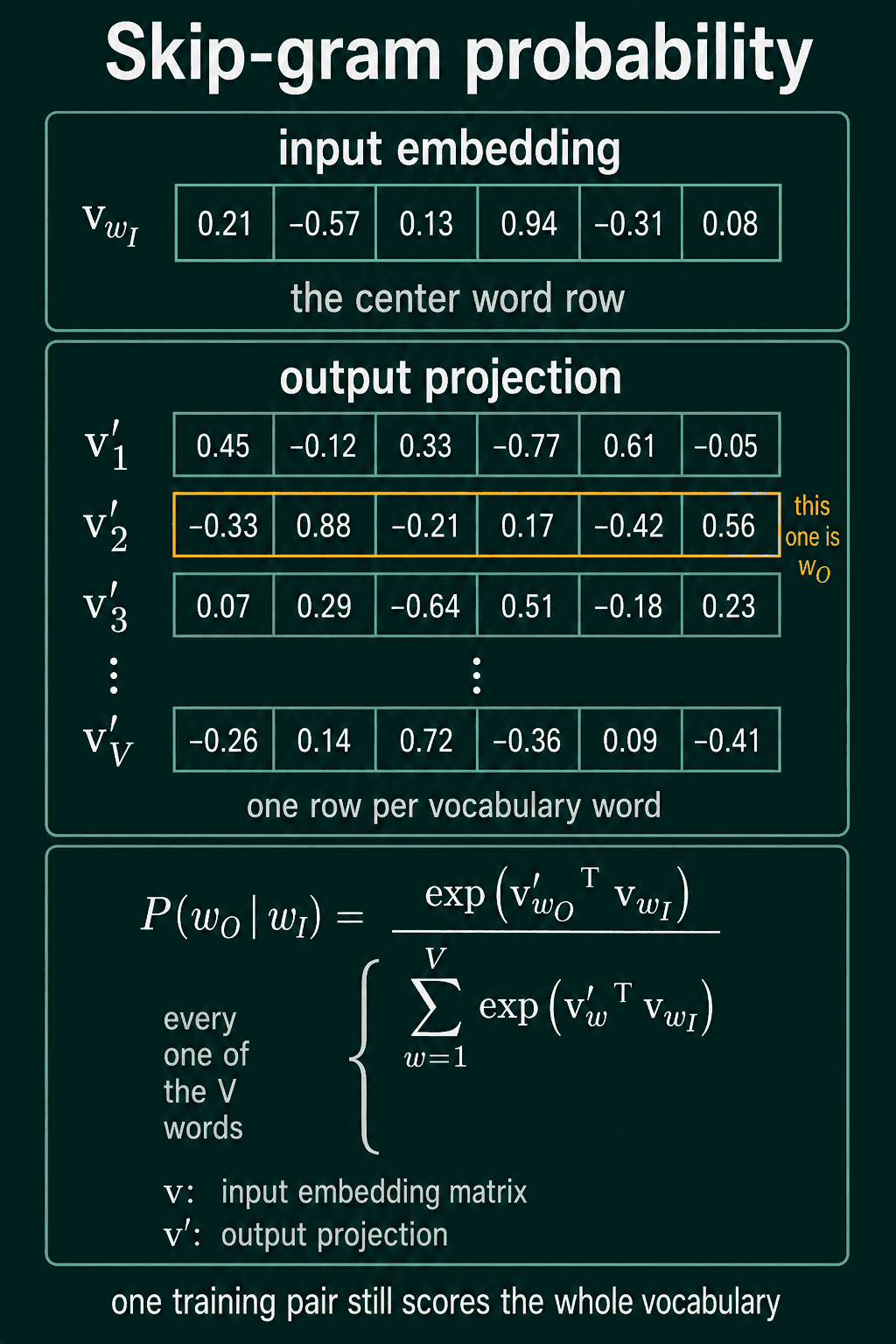
The Word2Vec formula writes the same idea with two sets of vectors. Each word has a row $\mathbf{v}$ in the embedding table and a row $\mathbf{v}'$ in the scoring layer. The score for a pair is their dot product, which multiplies matching entries and adds them up, so the dot product of $[1, 2]$ and $[3, 0]$ is $3$. Write $w_I$ for the input word, $w_O$ for one context word and $V$ for the vocabulary size:
$$P(w_O \mid w_I) = \frac{\exp(\mathbf{v}'^{\top}_{w_O} \mathbf{v}_{w_I})}{\sum_{w=1}^{V} \exp(\mathbf{v}'^{\top}_{w} \mathbf{v}_{w_I})}$$
The top is the score of the real context word. The bottom adds the scores of every word in the vocabulary, one dot product each, for every single training pair. That sum is the expensive part of training skip-gram. The PyTorch model uses nn.Linear, which adds a learned bias that this formula leaves out, and that is a small code convenience.
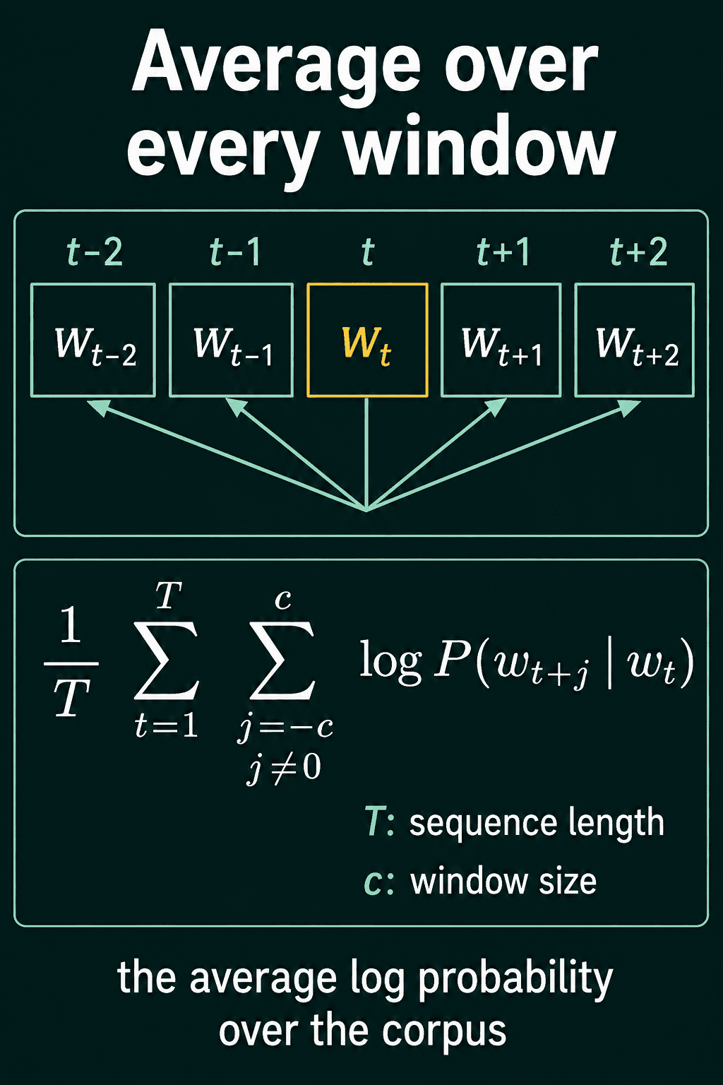
Across a whole text of $T$ words, skip-gram scores each context word in the window separately and adds the log probabilities. Training maximizes the average:
$$\frac{1}{T}\sum_{t=1}^{T} \sum_{-c \le j \le c,\ j \ne 0} \log P(w_{t+j} \mid w_t)$$
The inner sum runs over the window around position $t$ and skips the center itself. In the nine-word sentence above with $c = 2$, that comes to the 30 pairs the function printed.
Skip-gram in PyTorch
The model is an embedding lookup followed by a linear layer. This run trains it on the same sentence, one pair at a time:
1import torch.nn as nn
2
3class SkipGram(nn.Module):
4    def __init__(self, vocab_size, embedding_dim):
5        super().__init__()
6        self.embedding = nn.Embedding(vocab_size, embedding_dim)
7        self.linear = nn.Linear(embedding_dim, vocab_size)
8
9    def forward(self, center):
10        x = self.embedding(center)
11        return self.linear(x)
12
13torch.manual_seed(0)
14vocab = sorted(set(tokens))
15word_to_id = {word: i for i, word in enumerate(vocab)}
16id_pairs = [(word_to_id[c], word_to_id[o]) for c, o in pairs]
17
18model = SkipGram(vocab_size=len(vocab), embedding_dim=8)
19optimizer = torch.optim.SGD(model.parameters(), lr=0.1)
20
21for epoch in range(50):
22    total_loss = 0.0
23    for center, context in id_pairs:
24        logits = model(torch.tensor(center))
25        loss = F.cross_entropy(logits, torch.tensor(context))
26        optimizer.zero_grad()
27        loss.backward()
28        optimizer.step()
29        total_loss += loss.item()
30    if epoch in (0, 49):
31        print(epoch, round(total_loss / len(id_pairs), 3))
32
33embeddings = model.embedding.weight.detach()
34print(len(vocab), embeddings.shape)
It prints:
10 2.475
249 1.728
38 torch.Size([8, 8])
The average loss falls from 2.475 to 1.728. It cannot reach zero on this data, because "fox" has four correct context words and one softmax cannot give all four a probability of 1. Nine tokens also make eight distinct words, since "the" appears twice, so the table has 8 rows. A sentence this short only shows the code running. Useful vectors need far more text than this.
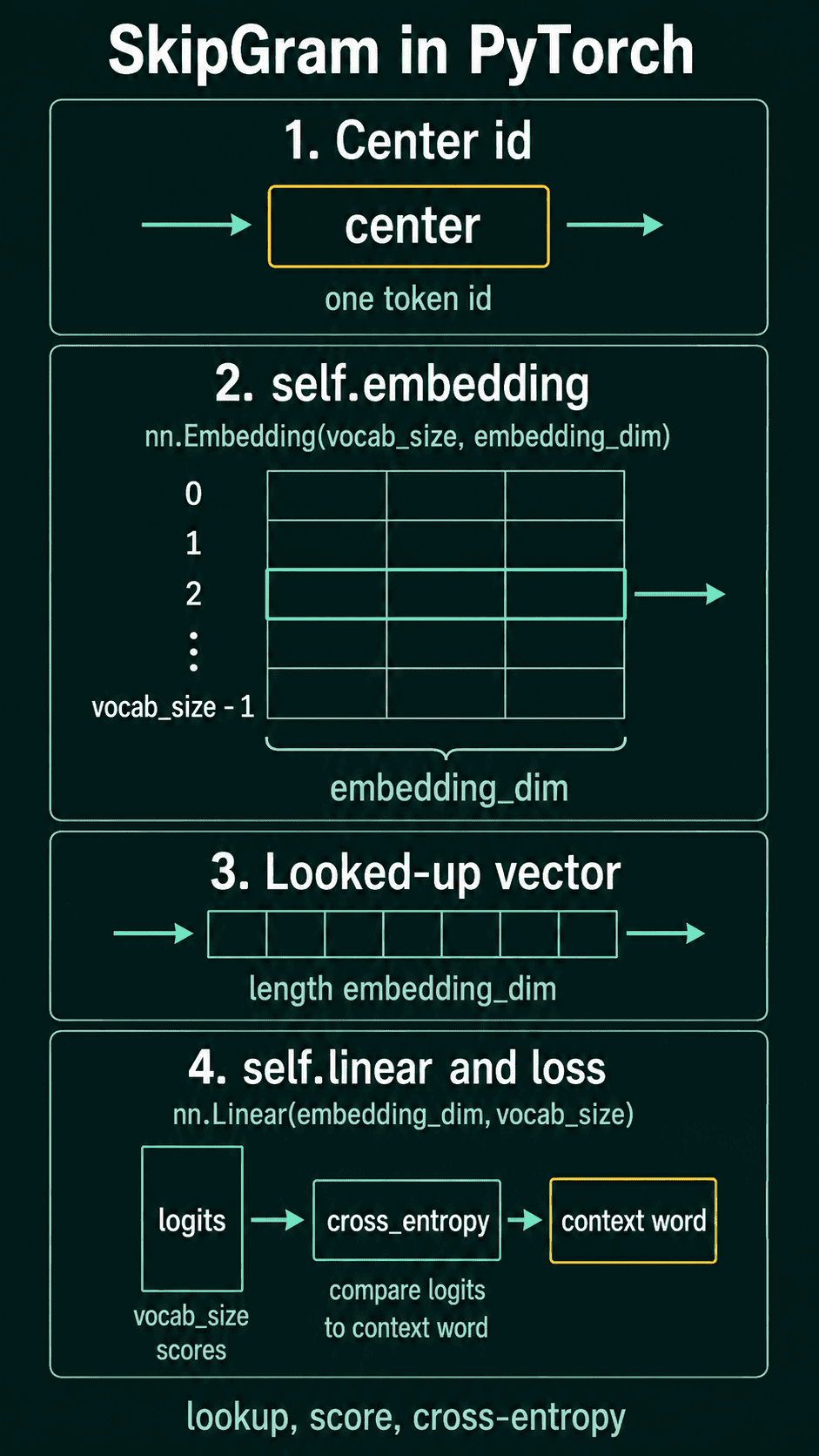
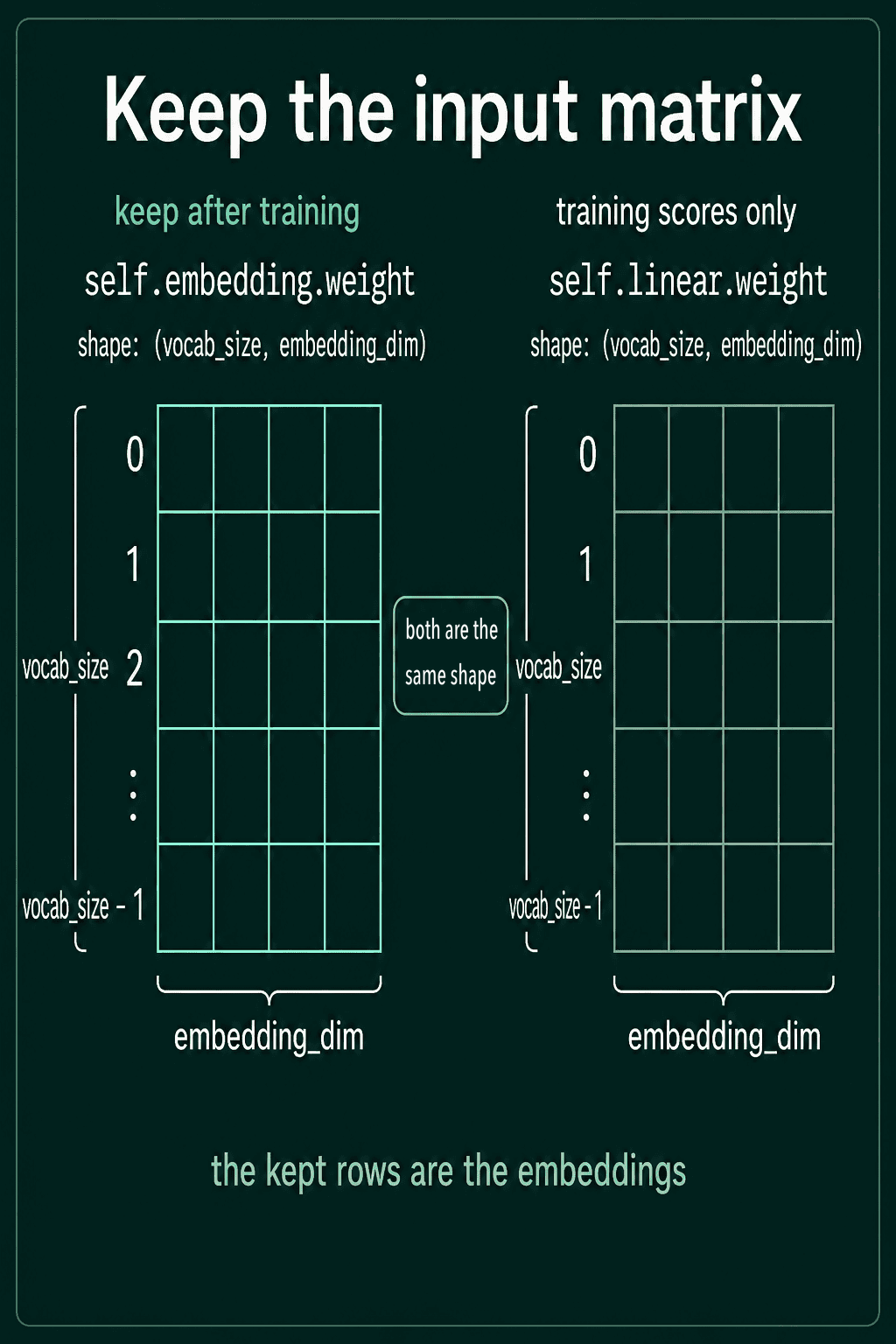
The network holds two matrices of the same shape. After training, model.embedding.weight is kept and its rows are the word embeddings. model.linear only produced the scores needed for the loss, so it is dropped.
CBOW: predict the center word from its context
CBOW stands for Continuous Bag of Words. It flips the direction and predicts the center word from the words around it. The four words "quick", "brown", "jumps" and "over" predict "fox".
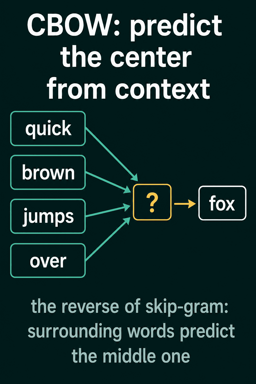
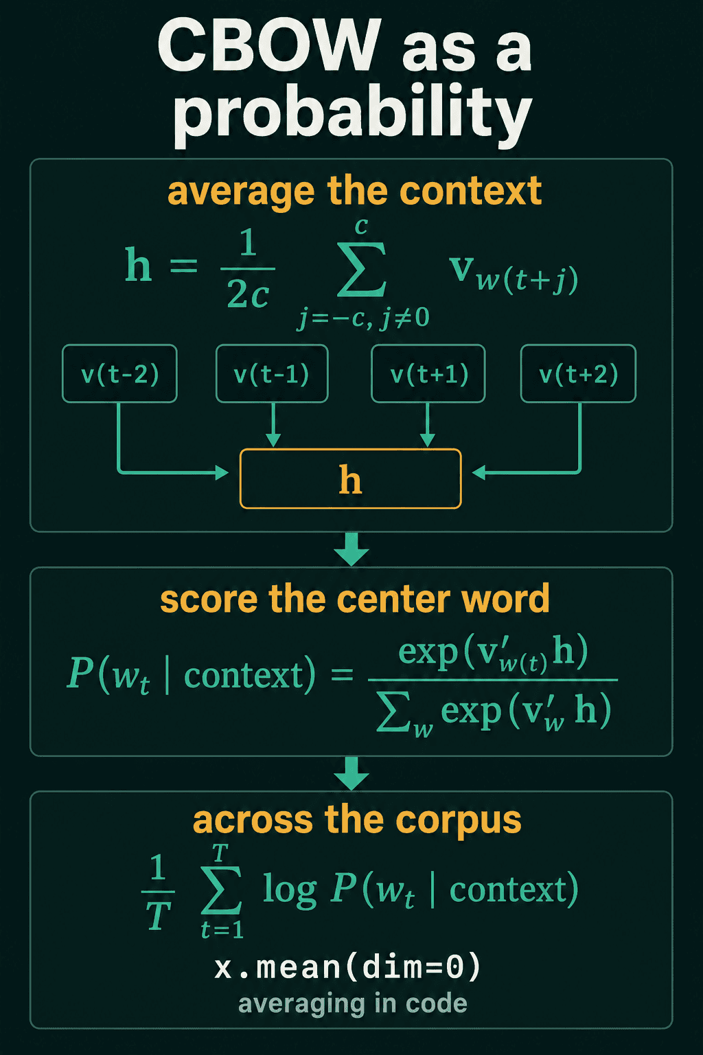
Skip-gram made one prediction per context word. CBOW makes one prediction per center word and uses all of the context words at once, by averaging their rows into a single vector $\mathbf{h}$:
$$\mathbf{h} = \frac{1}{2c} \sum_{-c \le j \le c,\ j \ne 0} \mathbf{v}_{w_{t+j}}$$
For example, with $c = 1$ there are two context words. If their rows are $[1, 0]$ and $[3, 2]$, then $\mathbf{h} = [2, 1]$.
The center word is then scored against every word in the vocabulary, the same way skip-gram scored a context word:
$$P(w_t \mid \text{context}_t) = \frac{\exp(\mathbf{v}'^{\top}_{w_t} \mathbf{h})}{\sum_{w=1}^{V} \exp(\mathbf{v}'^{\top}_{w} \mathbf{h})}$$
Across a text of $T$ words, CBOW maximizes the average log probability of the center word:
$$\frac{1}{T}\sum_{t=1}^{T} \log P(w_t \mid \text{context}_t)$$
CBOW needs its own pair function, because each example now holds a list of context words:
1def get_cbow_pairs(tokens, window_size):
2    pairs = []
3    end = len(tokens) - window_size
4    for i in range(window_size, end):
5        left = tokens[i - window_size:i]
6        right = tokens[i + 1:i + window_size + 1]
7        context = left + right
8        center = tokens[i]
9        pairs.append((context, center))
10    return pairs
11
12cbow_pairs = get_cbow_pairs(tokens, window_size=2)
13print(len(cbow_pairs))
14print(cbow_pairs[1])
It prints:
15
2(['quick', 'brown', 'jumps', 'over'], 'fox')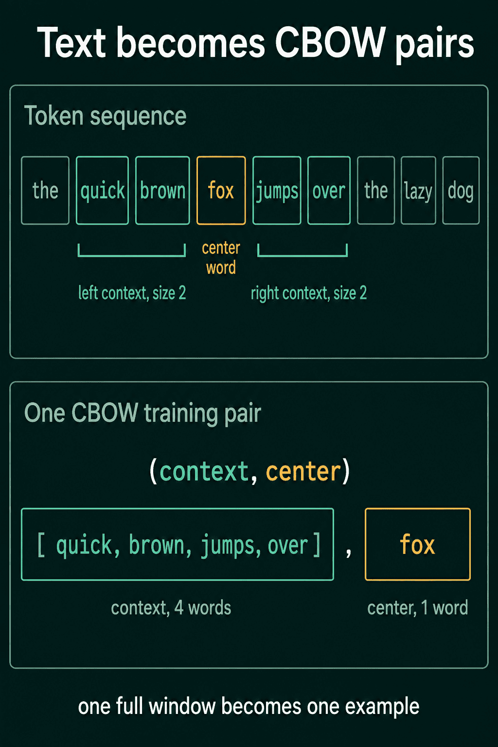
The nine-word sentence gives 5 examples here against 30 for skip-gram. i only covers positions with a full window on both sides. Positions 0, 1, 7 and 8 never become centers. The skip-gram function kept those edge words with a partial window.
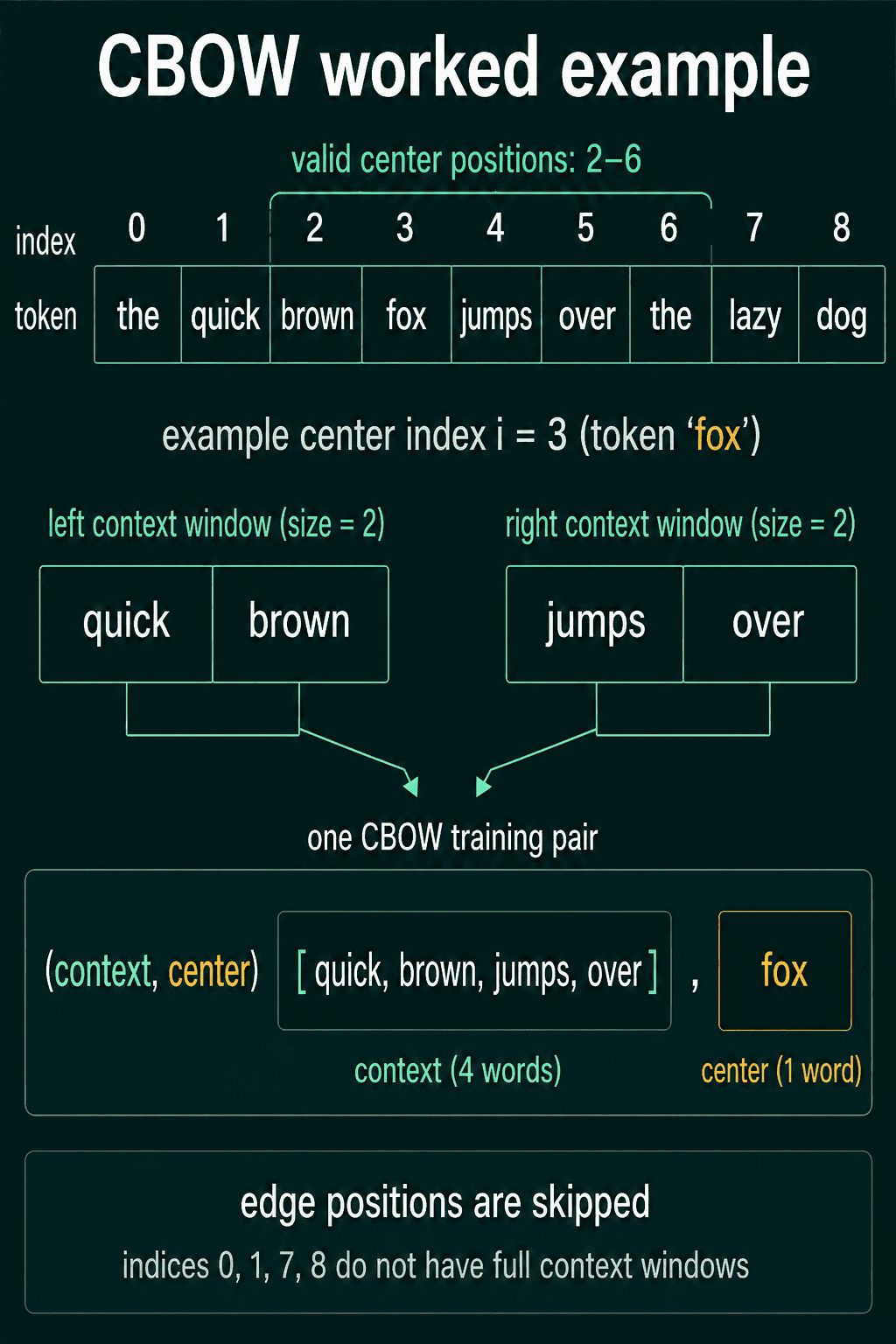
The model adds one line to skip-gram, the average:
1class CBOW(nn.Module):
2    def __init__(self, vocab_size, embedding_dim):
3        super().__init__()
4        self.embedding = nn.Embedding(vocab_size, embedding_dim)
5        self.linear = nn.Linear(embedding_dim, vocab_size)
6
7    def forward(self, context):
8        x = self.embedding(context)
9        x = x.mean(dim=0)
10        return self.linear(x)
11
12torch.manual_seed(0)
13model = CBOW(vocab_size=len(vocab), embedding_dim=8)
14context_words, center_word = cbow_pairs[1]
15context = torch.tensor([word_to_id[word] for word in context_words])
16target = torch.tensor(word_to_id[center_word]).unsqueeze(0)
17
18logits = model(context)
19print(model.embedding(context).shape, logits.shape)
20loss = F.cross_entropy(logits.unsqueeze(0), target)
21print(round(loss.item(), 3))
It prints:
1torch.Size([4, 8]) torch.Size([8])
22.047
The lookup returns 4 rows of length 8, one per context word. x.mean(dim=0) averages them into one vector of length 8, and the linear layer turns that into 8 scores. The target has shape (1,), so cross_entropy expects a batch of one, which is why logits gets .unsqueeze(0) before the loss.
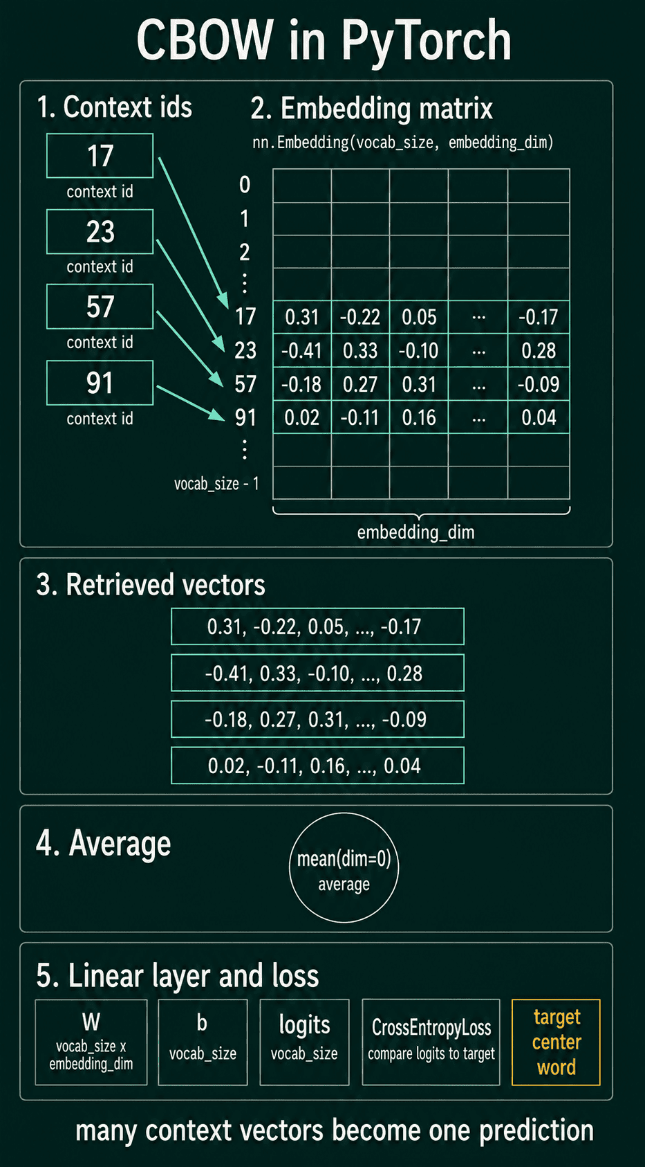
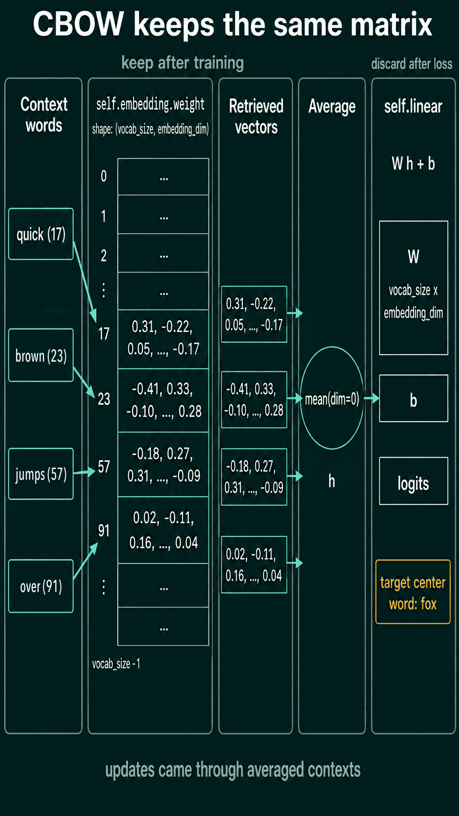
CBOW keeps the same matrix as skip-gram. After training, model.embedding.weight holds the embeddings and model.linear is dropped. What changes is how each row received its updates, since a word in CBOW usually gets updated as part of an averaged context.
Skip-gram vs CBOW
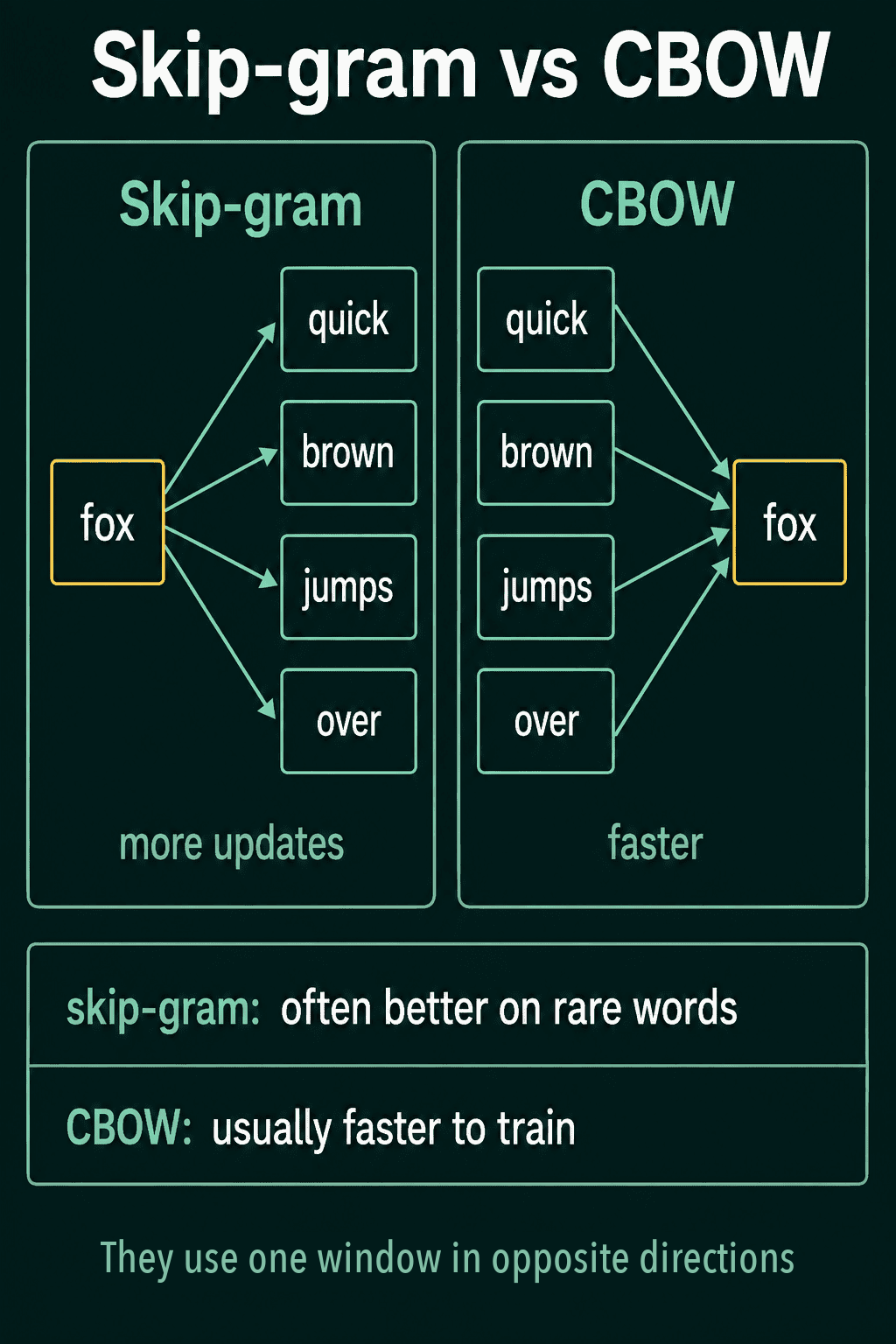
Both use the same window and the same embedding table, with the prediction running in opposite directions.
| Skip-gram | CBOW | |
|---|---|---|
| Input | center word | averaged context words |
| Predicts | each context word | center word |
| Predictions per center word | one per context word | one |
| Often chosen for | rare words | training speed |
Neither is the universal best choice. One occurrence of a word in skip-gram creates several training pairs, so rare words get more updates from the few times they appear. CBOW averages its context into one input and makes one prediction, which makes training faster. Skip-gram is often preferred when rare words need good vectors, and CBOW is a good baseline when training speed comes first.
Common mistakes
- Applying softmax before the loss.
F.cross_entropyexpects logits and runs the softmax step itself, so passing it probabilities computes the wrong loss with no error. Pass the raw output of the linear layer. - Keeping the wrong matrix. The embeddings are
model.embedding.weight. The weights inmodel.linearhave the same shape, so grabbing them also runs without an error. - Forgetting the CBOW shape.
x.mean(dim=0)leaves one vector of scores, whilecross_entropywith a target of shape(1,)expects a batch of scores. Add.unsqueeze(0)to the logits. - Using a window larger than the text allows.
get_cbow_pairsneeds $2c + 1$ tokens for a single example. With fewer than that it returns an empty list, so check the pair count before training.
Related concepts
The sum over every vocabulary word makes full softmax slow on a large vocabulary. Negative sampling and hierarchical softmax are the two common ways around it. GloVe and fastText learn word vectors from counts and from pieces of words. The post on word embeddings covers the embedding table itself, and the post on bag of words, co-occurrence matrices and PMI covers the counting route.
QuiddityML teaches Word2Vec, skip-gram and CBOW as separate concepts in the word representations unit of its NLP track, and the exercises include writing the pair functions from scratch and spotting the bug in a skip-gram loss (QuiddityML).