By Sagi Shaier · 31 October 2026 · 8 min read
Word2Vec vs GloVe vs fastText
What each word embedding method trains on, what its loss looks like in PyTorch, and how to pick one when your text has rare or unseen words.
Word2Vec, GloVe and fastText are three ways to learn word embeddings, the short lists of numbers that stand for words inside a model. All three start from the same signal, which is which words appear near each other. Word2Vec learns by predicting nearby words, GloVe learns from a table of word pair counts, and fastText builds each word out of pieces of letters so that it can handle words it never saw in training.
| Method | Trains on | Has a row for | Word not in training |
|---|---|---|---|
| Word2Vec | local windows | each whole word | no vector |
| GloVe | global pair counts | each whole word | no vector |
| fastText | local windows | letter pieces and whole words | built from pieces |
How does Word2Vec learn?
Word2Vec trains a small neural network to predict words from a window around each position in the text. Its skip-gram version takes a center word and predicts the words around it. Each word has a row in an embedding table, and training updates those rows one prediction at a time. The rows are the embeddings. The skip-gram and CBOW post walks through it with code.
How does GloVe learn?
Word2Vec reads the text one window at a time. GloVe, short for Global Vectors, counts first. It goes through the whole text once and builds a co-occurrence matrix $X$, where $X_{ij}$ is how often word $j$ appears in the context of word $i$.
Then it gives each word a word vector $\mathbf{w}_i$, a context vector $\tilde{\mathbf{w}}_j$ and two single numbers called biases, $b_i$ and $\tilde{b}_j$. Training changes those values until the vectors predict the log of the count:
$$\mathbf{w}_i^\top \tilde{\mathbf{w}}_j + b_i + \tilde{b}_j \approx \log X_{ij}$$
For example, say a pair of words appeared together 20 times, so the target is $\log 20 = 3.0$. Take $\mathbf{w}_i = [1, 0.5]$ and $\tilde{\mathbf{w}}_j = [2, 1]$, with biases $b_i = 0.2$ and $\tilde{b}_j = 0.1$. The dot product is 2.5 and the biases add 0.3, so the prediction is 2.8. The gap to the target is 0.2, and training shrinks it.
The full loss adds up the squared gap over word pairs, with a weight $f$ for each pair:
$$J = \sum_{i,j} f(X_{ij})\,\big(\mathbf{w}_i^\top \tilde{\mathbf{w}}_j + b_i + \tilde{b}_j - \log X_{ij}\big)^2$$
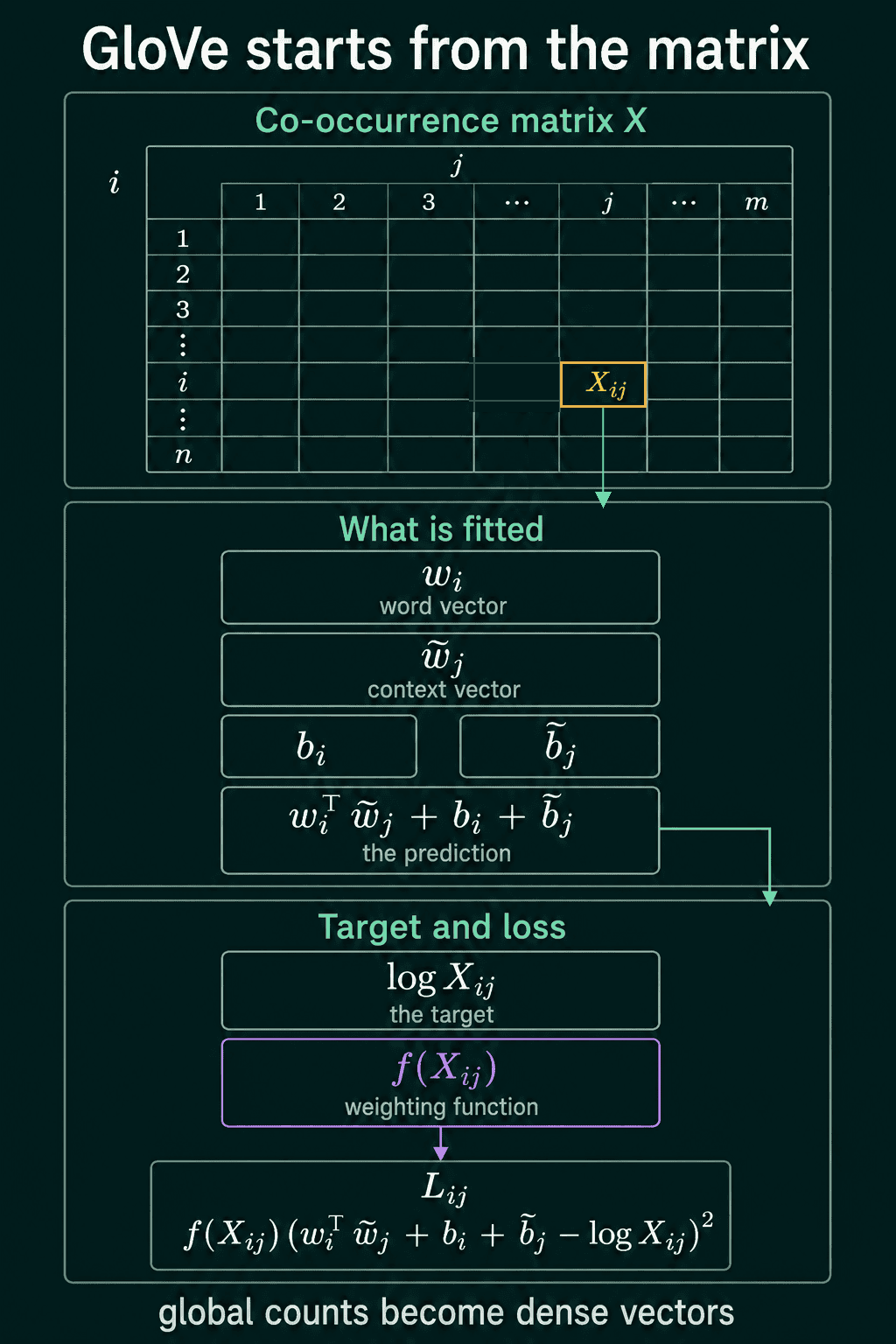
After training, the final embedding for a word is usually $\mathbf{w} + \tilde{\mathbf{w}}$, the word row plus the context row of that same word.
Why does GloVe fit log counts?
A single count is noisy, and the ratio of two probabilities can carry a cleaner signal. Compare how often a probe word $x$ appears near "dog" with how often it appears near "cat", which is $P(x \mid \text{dog}) / P(x \mid \text{cat})$.
When $x$ is "bark", the ratio is large. When $x$ is "purr", it is small. When $x$ is "pet", both animals share it and the ratio sits near 1. The word "sofa" is tied to neither, so it also lands near 1. The ratio keeps the words that separate "dog" from "cat" and cancels the ones they have in common.
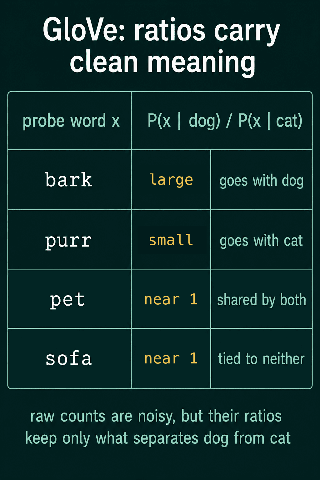
GloVe turns that into a formula by asking for vectors where $\exp(\mathbf{w}_i^\top \tilde{\mathbf{w}}_k)$ is proportional to the count $X_{ik}$. A ratio of two counts then becomes a difference of dot products, $(\mathbf{w}_i - \mathbf{w}_j)^\top \tilde{\mathbf{w}}_k$. Taking logs on both sides leaves $\mathbf{w}_i^\top \tilde{\mathbf{w}}_k \approx \log X_{ik}$, with the biases absorbing the row and column totals.
How does GloVe weight each pair?
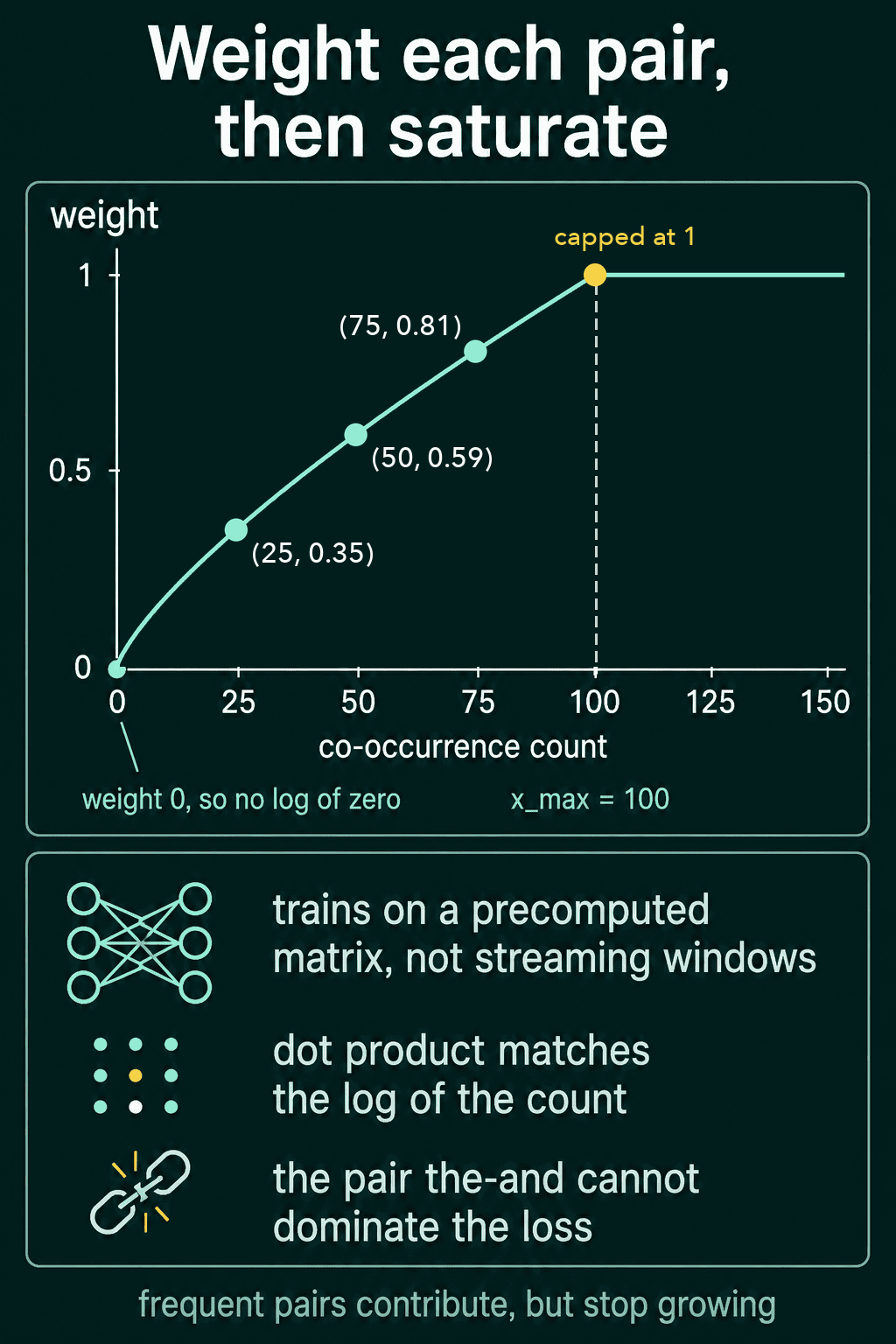
Very frequent pairs would take over the loss if every pair counted the same, so a weighting function scales each one:
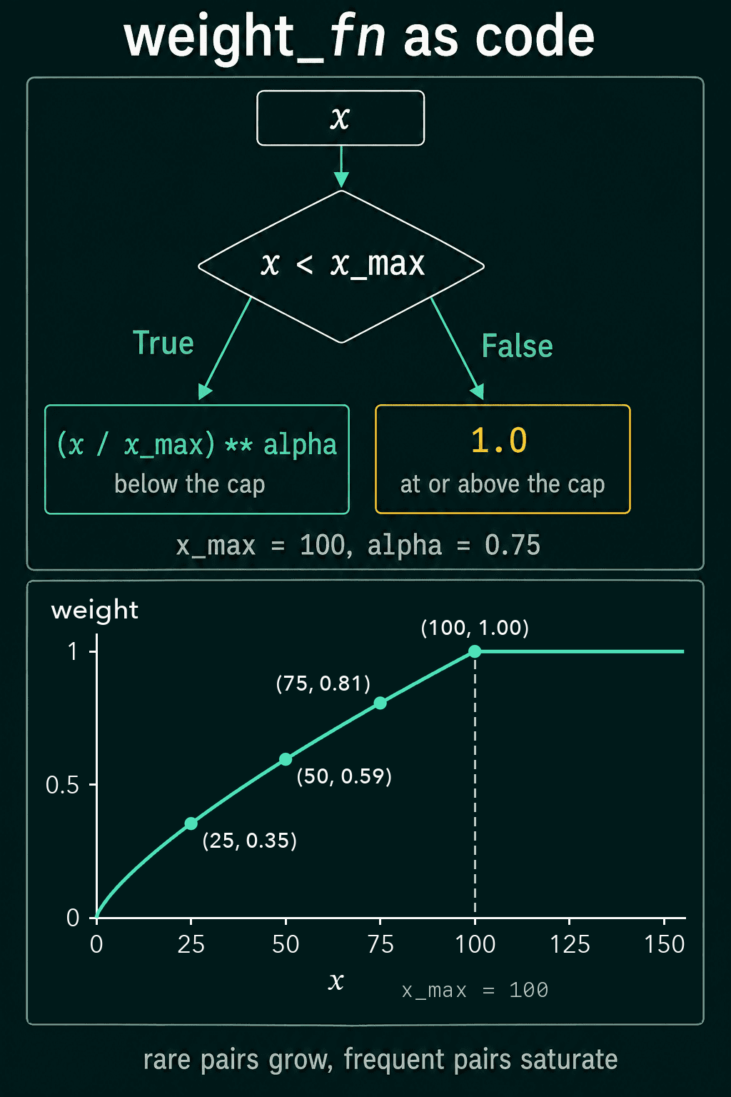
$$f(x) = \begin{cases}(x/x_{\max})^{\alpha} & x < x_{\max}\\ 1 & \text{otherwise}\end{cases}$$
The usual settings are $x_{\max} = 100$ and $\alpha = 0.75$. Pairs with a count of zero are left out of the sum entirely, because $\log 0$ is undefined. Here is the weight and the loss for one pair, using the numbers from the example above:
1import math
2import torch
3
4def weight_fn(x, x_max=100, alpha=0.75):
5    if x < x_max:
6        return (x / x_max) ** alpha
7    return 1.0
8
9def glove_loss(w_i, w_t_j, b_i, b_t_j, log_x_ij, weight):
10    pred = (w_i * w_t_j).sum() + b_i + b_t_j
11    return weight * (pred - log_x_ij) ** 2
12
13for count in (5, 20, 100, 400):
14    print(count, round(weight_fn(count), 3))
15
16w_i = torch.tensor([1.0, 0.5])
17w_t_j = torch.tensor([2.0, 1.0])
18loss = glove_loss(w_i, w_t_j, 0.2, 0.1, math.log(20), weight_fn(20))
19print(round(loss.item(), 4))
It prints:
15 0.106
220 0.299
3100 1.0
4400 1.0
50.0115
A pair seen 20 times gets a weight of 0.299, and a pair seen 400 times gets the same weight of 1.0 as one seen 100 times. So a pair like "the" next to a common word can only count so much.
The code follows the formula line by line. weight_fn branches on x_max, and glove_loss multiplies that weight by the squared gap between the predicted log count and the real one.
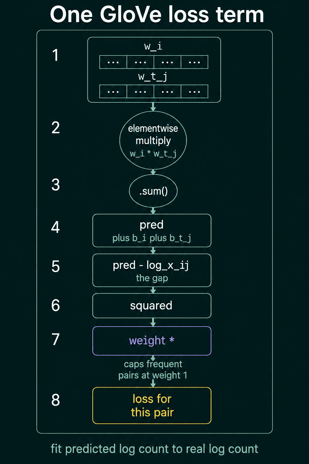
How does fastText handle unseen words?
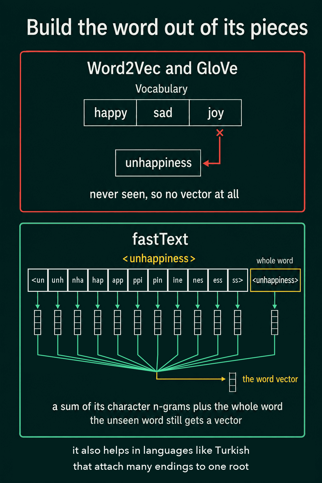
Word2Vec and GloVe share a blind spot. Each treats a word as one unit with its own row, so a word absent from training has no row to look up. This is the out-of-vocabulary problem.
fastText changes what gets a row. It trains vectors for character n-grams, the short overlapping runs of letters inside a word, and can also keep a vector for the whole word. It wraps each word in angle brackets to mark where it starts and ends, then reads off every overlapping run:
1def char_ngrams(word, n):
2    word = '<' + word + '>'
3    return [word[i:i + n] for i in range(len(word) - n + 1)]
4
5print(char_ngrams('jumping', 3))
6print(len(char_ngrams('unhappiness', 3)))
It prints:
1['<ju', 'jum', 'ump', 'mpi', 'pin', 'ing', 'ng>']
211
fastText keeps every n-gram from length 3 up to length 6, so one word carries short pieces like "jum" and longer ones like "jump" at the same time. This code stays at length 3 to keep it short.
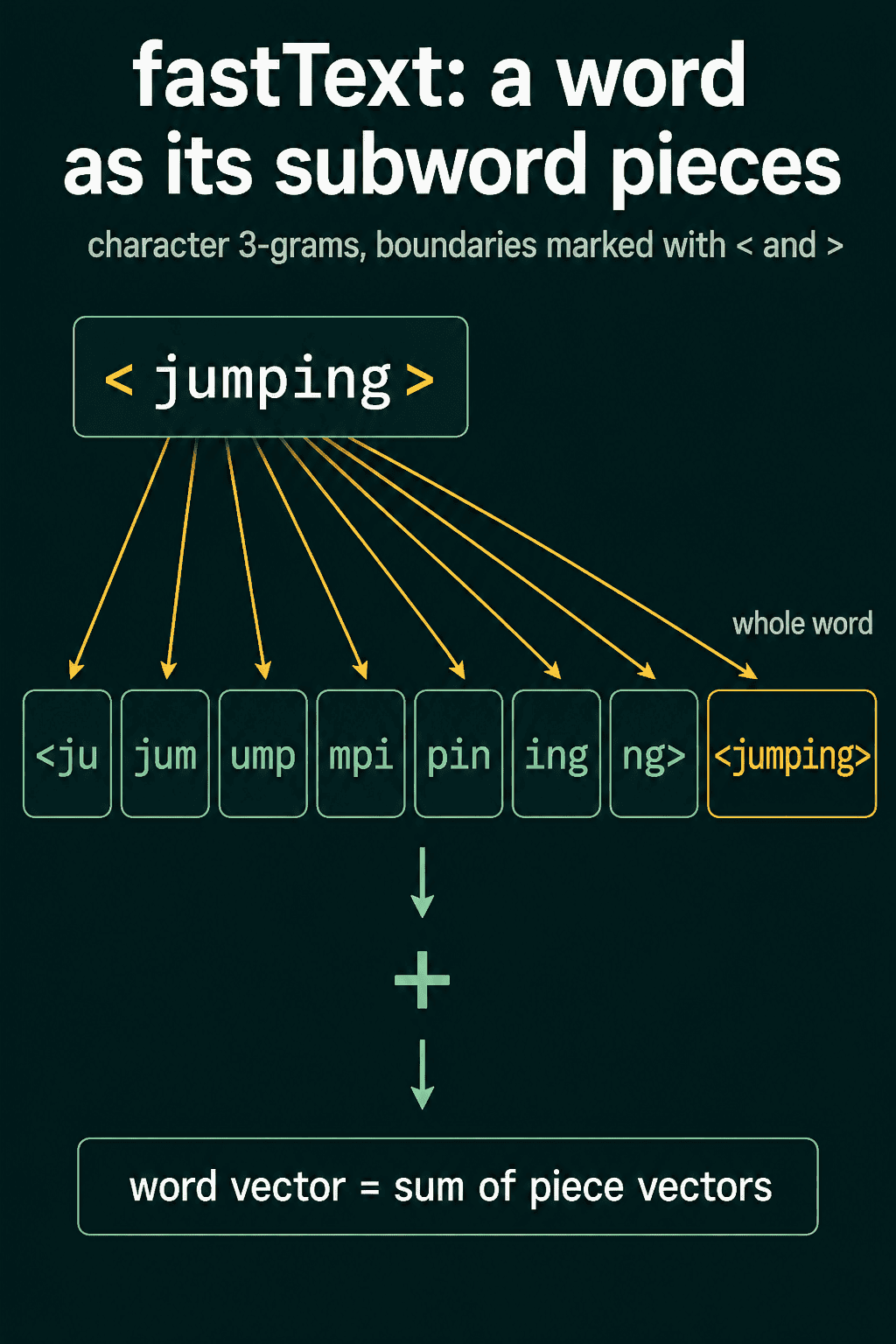
A word's vector is the sum of the rows of all its pieces. Different forms of one root overlap in their pieces and so pull toward each other. A word the model never saw can still be built out of pieces it shares with words it did see, so it gets a vector instead of none. This also helps in languages like Turkish that attach many endings to one root.
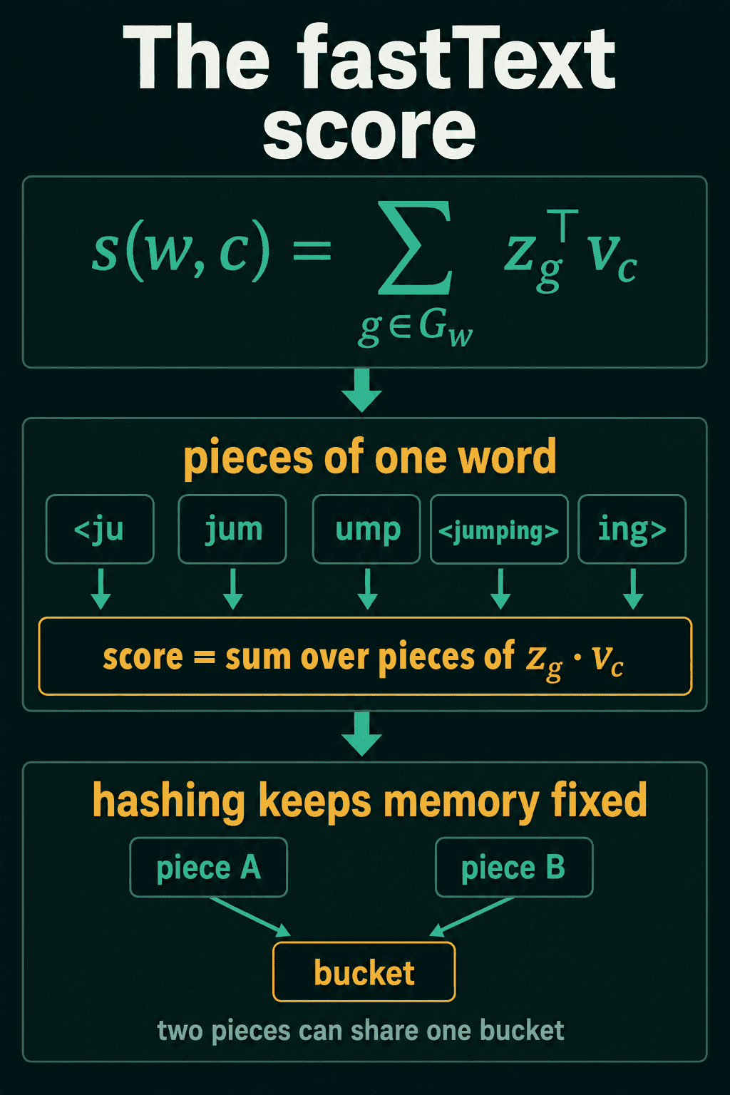
During training, the score for a word $w$ and a context word $c$ sums over all of its pieces. $G_w$ is the set of pieces of $w$, $\mathbf{z}_g$ is the vector for one piece $g$, and $\mathbf{v}_c$ is the context word's vector:
$$s(w, c) = \sum_{g \in G_w} \mathbf{z}_g^\top \mathbf{v}_c$$
That score goes into the skip-gram objective with negative sampling, so a real pair is pushed up and a few sampled pairs are pushed down.
Storing one vector per distinct piece would not fit in memory, since a large text produces millions of pieces. fastText hashes each piece into a table with a fixed number of rows called buckets. The memory cost is set in advance, and two pieces can land in the same bucket and share a row. This code builds that table with random rows, before any training:
1import zlib
2import torch.nn as nn
3
4torch.manual_seed(0)
5buckets = nn.Embedding(100_000, 50)
6
7def word_vector(word):
8    pieces = char_ngrams(word, 3) + ['<' + word + '>']
9    ids = [zlib.crc32(piece.encode()) % 100_000 for piece in pieces]
10    return buckets(torch.tensor(ids)).sum(dim=0)
11
12cosine = nn.CosineSimilarity(dim=0)
13print(round(cosine(word_vector('jump'), word_vector('jumped')).item(), 3))
14print(round(cosine(word_vector('jump'), word_vector('piano')).item(), 3))
15print(word_vector('unjumpable').shape)
It prints:
10.473
2-0.046
3torch.Size([50])
Cosine similarity measures how closely two vectors point the same way, from -1 to 1. With no training at all, "jump" and "jumped" already score 0.473 because they share the rows for <ju, jum and ump. The pair "jump" and "piano" scores near 0. A made-up word like "unjumpable" still gets a vector of length 50.
How are counting and predicting related?
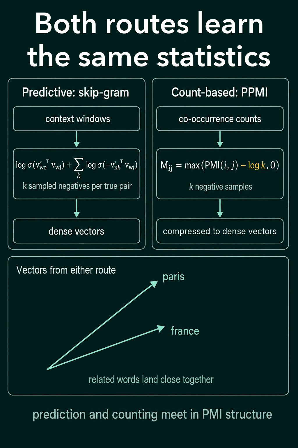
Word2Vec and the older counting methods are more closely related than they first look. PMI, or pointwise mutual information, measures how much more often two words appear together than chance would suggest. Skip-gram with negative sampling can be understood as implicitly factorizing a matrix of PMI values shifted by $\log k$, where $k$ is the number of negatives, under simplifying assumptions about the embedding size and the optimization.
In practice, predictive and count-based word vectors are two routes into the same statistics about which words appear together. One route counts first and compresses. The other trains a prediction model and lets its weights absorb the counts indirectly. GloVe sits in between, since it counts first and then trains.
Which one should you use?
- fastText is the one to reach for when your text has many words the model will not have seen. Typos and rare word forms are common cases, along with languages that attach many endings to one root. It is the only one of the three that gives those words a vector.
- GloVe suits a fixed text you can count once, because it trains on a precomputed matrix. Reading through the text again is not part of training.
- Word2Vec suits text you want to train on window by window. Its skip-gram version is often preferred when rare words need good vectors, and CBOW is a good baseline when training speed comes first.
All three give one vector per word, so "bank" gets the same vector in "river bank" and "bank account".
Common mistakes
- Taking the log of a zero count. GloVe's loss has no value for $X_{ij} = 0$, so those pairs must be left out of the sum.
- Keeping only the word vectors from GloVe. The final embedding is usually $\mathbf{w} + \tilde{\mathbf{w}}$, and dropping the context row throws half the training away.
- Expecting a Word2Vec or GloVe vector for a new word. Neither has a row for it, so a lookup fails. Check coverage on your own text first, and move to fastText if many words are missing.
- Assuming every fastText piece has its own row. Hashing can place two pieces in the same bucket. A larger table makes that rarer and costs more memory.
Related concepts
The post on negative sampling and hierarchical softmax covers the training shortcut fastText uses. The post on bag of words, co-occurrence matrices and PMI covers the counting that GloVe builds on, and the word embeddings post covers how to use the resulting table.
QuiddityML teaches GloVe and fastText as separate concepts in the word representations unit of its NLP track, and the exercises include writing GloVe's weighting function from its equation and spotting the bug in a character n-gram function (QuiddityML).