By Sagi Shaier · 9 October 2026 · 4 min read

Invariance vs equivariance, and why convolution is translation equivariant

The two equations that separate an invariant function from an equivariant one, worked examples with rotations and shifts, which network layers have which property, and PyTorch checks you can run on a convolution, a pooling step, and a shuffled hidden layer.

A function is invariant to a transformation when transforming its input leaves the output unchanged, and equivariant when transforming the input transforms the output in the same way. The two words describe how a network layer responds to a shifted or rotated input, and they explain why convolutional networks use convolution layers early on and pooling later.

The two definitions

Write the function as $f$, the input as $\mathbf{x}$, and the transformation (a rotation, a shift, a reflection) as $T$. $T(\mathbf{x})$ is the transformed input.

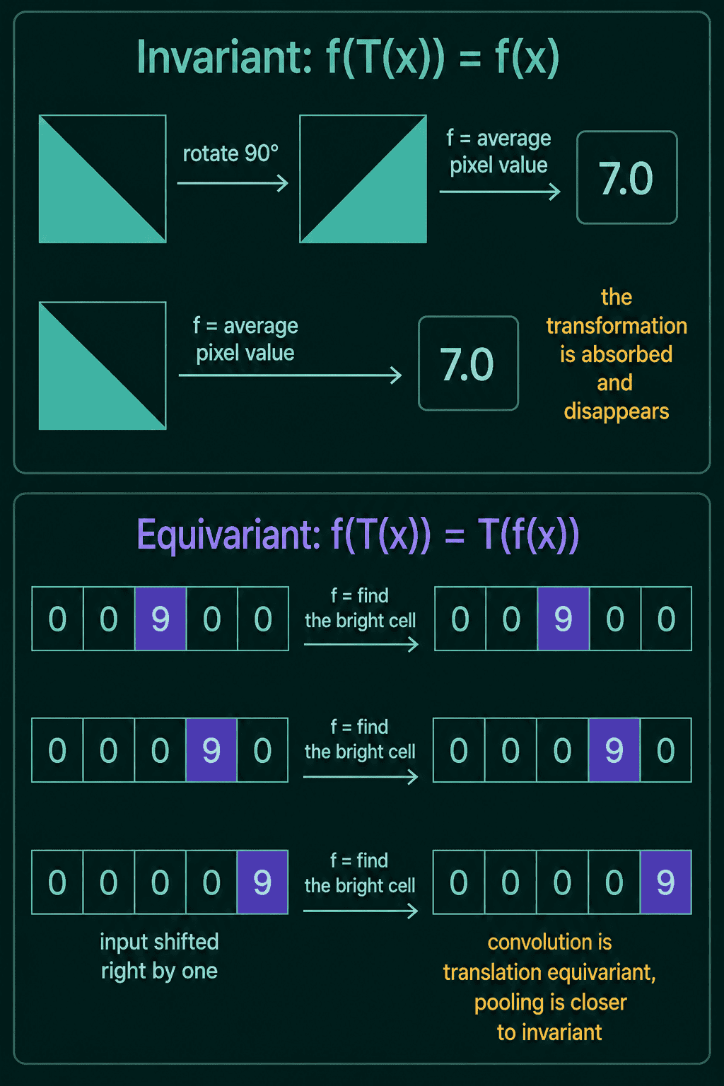
$f$ is invariant to $T$ when transforming the input first gives the same output as before:

$$f(T(\mathbf{x})) = f(\mathbf{x})$$

$f$ is equivariant to $T$ when transforming the input first gives the original output, transformed the same way:

$$f(T(\mathbf{x})) = T(f(\mathbf{x}))$$

Under invariance the transformation disappears from the output. Under equivariance it passes through to the output.

A worked example with rotations

A rotation matrix $Q$ turns a vector by some angle and keeps its length. Two functions show the difference.

Length is invariant to rotation. With $f(\mathbf{x}) = \|\mathbf{x}\|$, rotating first gives $\|Q\mathbf{x}\| = \|\mathbf{x}\|$, the same number, and the rotation leaves no trace in the output.

Scaling is equivariant to rotation. With $f(\mathbf{x}) = 3\mathbf{x}$, rotating first gives $3Q\mathbf{x}$, which equals $Q(3\mathbf{x}) = Q f(\mathbf{x})$: the output is the original output, rotated.

Images give the same contrast. Rotate an image and its average pixel value stays the same, so average brightness is invariant to rotation. Rotate an image and the edges found inside it rotate with it, so edge detection is equivariant to rotation.

Top: an image rotated by 90 degrees has the same average pixel value of 7.0 before and after, so the average is invariant. Bottom: a row of cells with one bright cell, shifted right by one, gives an output whose bright cell also shifts right by one, so the function is equivariant

Where each property shows up in a network

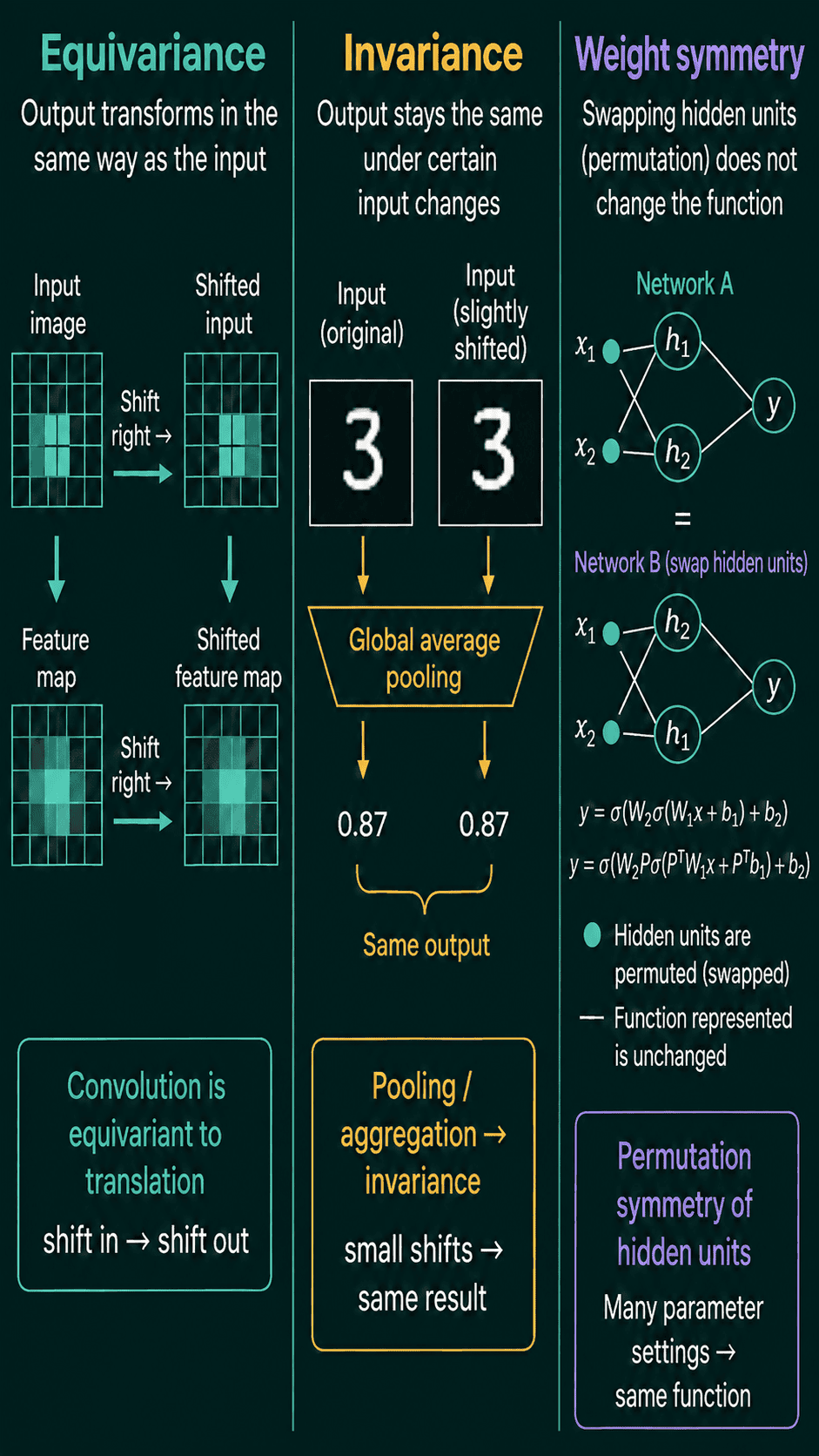
A convolution layer slides a small filter across its input and computes one output value per position. The same filter is used at every position, so shifting the input sideways shifts the output (called a feature map) by the same amount. Convolution is translation equivariant, where translation means a shift.

A pooling layer takes the maximum or the average over a region. A small shift in where a feature sits barely changes the pooled value, so pooling is close to translation invariant. Pooling over the whole feature map, called global pooling, ignores the position of a feature entirely.

Networks use the two properties for different jobs. Early convolution layers keep track of where things are, which is equivariance. Later pooling layers stop caring about small shifts once a feature has been found, which is invariance.

Three columns: a convolution whose feature map shifts right when its input image shifts right, global average pooling that gives 0.87 for both an original and a slightly shifted digit, and two small networks with their two hidden units swapped that compute the same function

Symmetries in the weights

A symmetry of an object is a transformation that leaves it unchanged. Networks have symmetries in their own weights. Take one hidden layer and reorder its neurons, moving each neuron's incoming weights, its bias, and its outgoing weights together. The network computes exactly the same function, so the loss is invariant to that reordering, even though the weight matrices now look different. Most functions are neither invariant nor equivariant to a given transformation, which is why architectures are designed to have one or the other.

Checking both properties in PyTorch

1import torch
2import torch.nn.functional as F
3 
4torch.manual_seed(0)
5img = torch.rand(8, 8)
6 
7# invariant: the average pixel value ignores a 90 degree rotation
8print(img.mean(), torch.rot90(img).mean())
9 
10# equivariant: shifting the input shifts a convolution's output
11signal = torch.tensor([0., 0., 1., 3., 1., 0., 0., 0., 0., 0.])
12kernel = torch.tensor([1., -1.])
13conv = lambda s: F.conv1d(s.view(1, 1, -1), kernel.view(1, 1, -1)).view(-1)
14shifted = torch.roll(signal, 2)
15print(conv(signal))
16print(conv(shifted))
17print(torch.roll(conv(signal), 2))
18 
19# global max pooling: the shift disappears from the output
20print(conv(signal).max(), conv(shifted).max())

1tensor(0.4703) tensor(0.4703)
2tensor([ 0., -1., -2.,  2.,  1.,  0.,  0.,  0.,  0.])
3tensor([ 0.,  0.,  0., -1., -2.,  2.,  1.,  0.,  0.])
4tensor([ 0.,  0.,  0., -1., -2.,  2.,  1.,  0.,  0.])
5tensor(2.) tensor(2.)

torch.roll(signal, 2) shifts the signal two places to the right. Convolving the shifted signal gives the same output as shifting the convolved signal, which is the equivariance equation $f(T(\mathbf{x})) = T(f(\mathbf{x}))$. Taking the max over all positions gives 2 for both, which is the invariance equation. The bump in this signal sits away from the edges on purpose: near an edge, padding and the shifted-in zeros break exact equivariance, so if a check like this fails, look at the borders first.

Reordering hidden neurons, with their weights moved together:

1import torch
2 
3torch.manual_seed(0)
4net = torch.nn.Sequential(torch.nn.Linear(2, 3), torch.nn.ReLU(), torch.nn.Linear(3, 1))
5x = torch.randn(4, 2)
6before = net(x)
7 
8perm = torch.tensor([2, 0, 1])                    # reorder the 3 hidden neurons
9with torch.no_grad():
10    net[0].weight.copy_(net[0].weight[perm])
11    net[0].bias.copy_(net[0].bias[perm])
12    net[2].weight.copy_(net[2].weight[:, perm])
13after = net(x)
14print(torch.allclose(before, after))

1True

The rows of the first layer's weights and bias are reordered, and the columns of the second layer's weights are reordered the same way, so each hidden neuron keeps its own inputs and outputs.

Common mistakes

Using the two words interchangeably. An invariant output does not change, and an equivariant output changes in step with the input.
Calling convolution translation invariant. A convolution's output moves when the input moves, and it takes pooling to remove the position.
Expecting equivariance to hold at the borders. Padding and cropping at the edges make the property approximate there.
Assuming equivariance to one transformation gives it for others. A plain convolution is equivariant to shifts, not to rotations.

Orthogonal matrices are the rotations and reflections, and lengths are invariant to them, covered in orthogonality explained. Vector norms, the lengths used in the rotation example, are in vector norms and distances.

QuiddityML teaches invariance and equivariance as their own concept in the linear algebra part of the Math track, and the exercises include telling the two apart for rotations and shifts, ordering the lines of an is_shift_equivariant check, and writing that check from scratch.