By Sagi Shaier · 8 October 2026 · 6 min read
Rank, column space and null space explained
How to find the rank of a matrix by hand, what the column space and null space say about whether Ax = b has a solution, why a large weight matrix can hold far fewer independent directions than its size, and how to check all of it in PyTorch.
The rank of a matrix is the number of independent directions among its rows, which is always the same as the number among its columns. A $3 \times 3$ matrix can have rank 3, 2, 1 or 0, and the rank says how many dimensions survive when the matrix transforms a vector. The column space is the set of every output the matrix can produce, and the null space is the set of every input it sends to zero.
Rank: how many dimensions survive
A set of vectors is linearly independent when none of them can be built by scaling and adding the others. The rank of a matrix $A$ is the number of linearly independent rows it has, and the number of independent columns always comes out the same.
A $3 \times 3$ matrix whose three rows are independent has rank 3: nothing collapses, and its outputs fill all of 3D space. If one row is a combination of the other two, the rank drops to 2, and every output lands on a flat plane inside 3D space, even though the matrix still has 3 rows. If every row is a multiple of one row, the rank is 1, and every output lands on a single line.
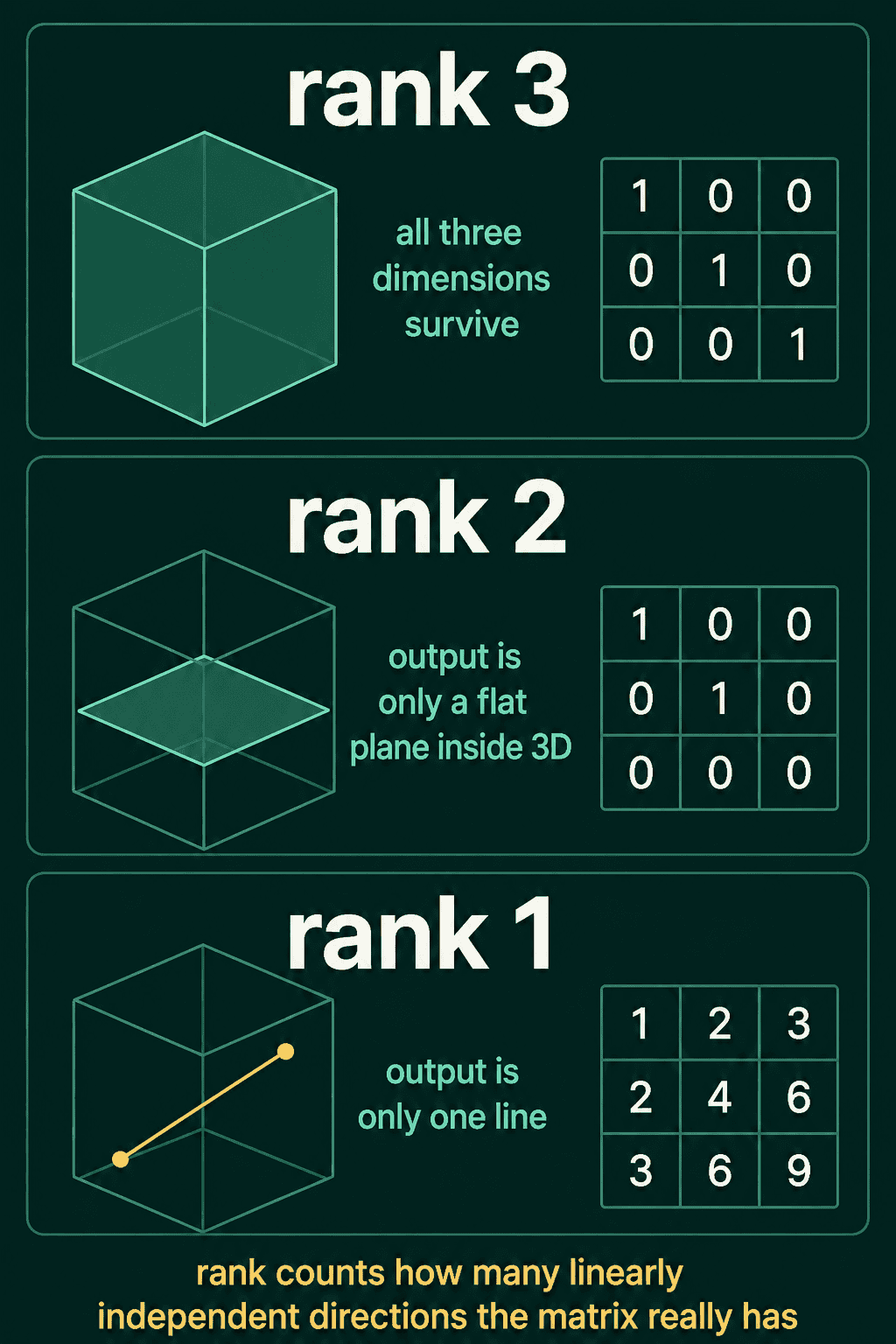
A matrix whose rank equals the smaller of its row count and column count has full rank. A matrix with less than that is rank-deficient. For a square matrix, rank-deficient means the same thing as having a determinant of 0, which means the matrix is singular and has no inverse.
Finding the rank by hand
Gaussian elimination finds the rank: use the row operations (swap two rows, scale a row by a nonzero number, add a multiple of one row to another) to clear entries below each leading entry, then count the rows that are not all zeros. Take
$$A = \begin{bmatrix} 1 & 2 & 3 \ 2 & 4 & 6 \ 1 & 1 & 1 \end{bmatrix}$$
Row 2 is exactly twice row 1, so subtracting $2 \times$ row 1 from row 2 turns it into $[,0\ \ 0\ \ 0,]$. Subtracting row 1 from row 3 turns it into $[,0\ \ -1\ \ -2,]$. Swapping the bottom two rows gives
$$\begin{bmatrix} 1 & 2 & 3 \ 0 & -1 & -2 \ 0 & 0 & 0 \end{bmatrix}$$
Two rows are not all zeros, so the rank is 2.
Rank in machine learning
A weight matrix of size $1000 \times 1000$ can have rank 50, which means the other 950 dimensions hold only combinations of the first 50 and add no new independent information. One common way to fine-tune a large pretrained model, called LoRA, uses this directly: instead of updating a full weight matrix, it learns a low-rank update, on the bet that the needed change does not use all the dimensions.
Three rules limit what rank can do. A product never gains rank:
$$\text{rank}(AB) \leq \min(\text{rank}(A), \text{rank}(B))$$
so a $100 \times 2$ matrix times a $2 \times 100$ matrix gives a $100 \times 100$ result with rank at most 2. Transposing leaves rank unchanged, $\text{rank}(A^\top) = \text{rank}(A)$. And a sum has at most the combined rank of its parts:
$$\text{rank}(A + B) \leq \text{rank}(A) + \text{rank}(B)$$
Column space: every output A can produce
The column space of $A$ is the span of its columns: every vector you can get by scaling the columns and adding them, which is exactly every output $A\mathbf{x}$ over all possible inputs $\mathbf{x}$.
The column space is a subspace, a flat set of vectors through the origin where adding two members or scaling one always gives another member. A line through the origin is a subspace, so is a plane through the origin, and so is the whole space. A line that misses the origin is not.
The dimension of the column space is the rank. A rank-2 matrix that outputs 3D vectors has a column space that is a 2D plane inside 3D space. Any target $\mathbf{b}$ off that plane cannot be reached, so $A\mathbf{x} = \mathbf{b}$ has no solution for it.
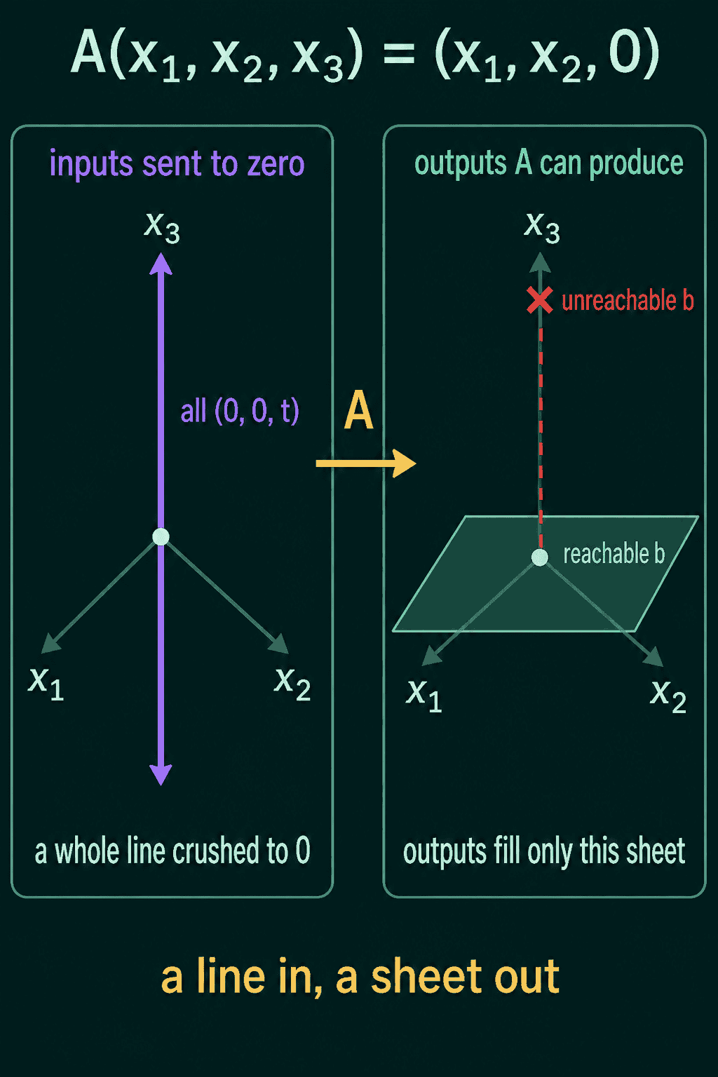
The matrix in that picture keeps the first two coordinates and replaces the third with 0, so its outputs fill the flat plane where the third coordinate is 0, and any $\mathbf{b}$ with a nonzero third coordinate is out of reach.
Null space: every input A sends to zero
The null space of $A$ is the set of inputs that $A$ maps to the zero vector:
$$\text{null}(A) = {\mathbf{x} : A\mathbf{x} = \mathbf{0}}$$
For a square full-rank matrix, the only such input is the zero vector itself. For a rank-deficient matrix there is a whole subspace of nonzero inputs that get squashed to zero, which are the directions the transformation destroys. In the picture above that is the $x_3$ axis.
A nonzero null space is what makes "infinitely many solutions" possible. If $A\mathbf{x}_0 = \mathbf{b}$ for one solution $\mathbf{x}_0$, then adding any vector from the null space to $\mathbf{x}_0$ gives another solution, because that added part contributes nothing to the output.
Rank-nullity: how the two dimensions add up
One identity ties rank and null space together:
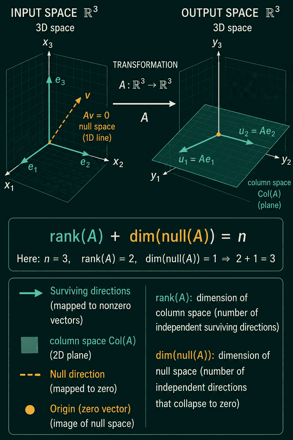
$$\text{rank}(A) + \dim(\text{null}(A)) = n$$
Here $n$ is the number of columns of $A$, which is the number of input directions, and $\dim(\text{null}(A))$ is the dimension of the null space. Every input direction either survives into the column space or collapses into the null space. A $3 \times 4$ matrix of rank 3 has a 1-dimensional null space, so its solutions come as a whole line instead of a single point.
Rank, column space and null space in PyTorch
1import torch
2
3torch.manual_seed(0)
4
5I3 = torch.eye(3)
6P = torch.tensor([[1., 0., 0.],
7                  [0., 1., 0.],
8                  [0., 0., 0.]])
9R1 = torch.tensor([[1., 2., 3.],
10                   [2., 4., 6.],
11                   [3., 6., 9.]])
12print(torch.linalg.matrix_rank(I3), torch.linalg.matrix_rank(P), torch.linalg.matrix_rank(R1))
13
14A = torch.tensor([[1., 2., 3.],
15                  [2., 4., 6.],
16                  [1., 1., 1.]])
17print(torch.linalg.matrix_rank(A))
18
19# null space: x = (1, -2, 1) is sent to the zero vector
20x = torch.tensor([1., -2., 1.])
21print(A @ x)
22
23# rank-nullity: dim(null) = number of columns - rank
24n = A.shape[1]
25print(n - torch.linalg.matrix_rank(A).item())
26
27# column space: every output has second entry = 2 * first entry
28for _ in range(3):
29    y = A @ torch.randn(3)
30    print(y[1] / y[0])
31
32# a product never gains rank
33tall = torch.randn(100, 2)
34wide = torch.randn(2, 100)
35print(torch.linalg.matrix_rank(tall @ wide), (tall @ wide).shape)1tensor(3) tensor(2) tensor(1)
2tensor(2)
3tensor([0., 0., 0.])
41
5tensor(2.)
6tensor(2.)
7tensor(2.)
8tensor(2) torch.Size([100, 100])Since row 2 of $A$ is twice row 1, every output $A\mathbf{x}$ has a second entry equal to twice its first, which is the plane the column space lives on, so a target like $(1, 0, 0)$ can never be reached. The vector $(1, -2, 1)$ is in the null space, and rank-nullity says the null space is 1-dimensional, so every null-space vector is a multiple of it. When a matrix behaves strangely, comparing torch.linalg.matrix_rank with its smaller dimension is a quick first check.
Common mistakes
- Reading rank off the shape. A $1000 \times 1000$ matrix can have rank 50, and only the rank says how many directions are independent.
- Mixing up the two spaces. The column space lives among the outputs, and the null space lives among the inputs.
- Using the row count in rank-nullity. The $n$ in $\text{rank}(A) + \dim(\text{null}(A)) = n$ is the number of columns.
- Expecting a product to recover rank. $\text{rank}(AB)$ is at most the smaller of the two ranks, so a narrow middle dimension caps the result.
Related math
Span, basis and linear independence, the ideas rank is built on, are covered in span, basis and linear independence. The determinant and inverse, the yes-or-no version of the same question for square matrices, are in determinant, inverse and trace explained.
QuiddityML teaches rank and the column and null spaces as two concepts in the linear algebra part of the Math track, and the exercises include tracing a rank and null-dimension count for a $3 \times 5$ matrix and writing an in_null_space check that tests whether $A\mathbf{x}$ is close to zero.