By Sagi Shaier · 7 October 2026 · 5 min read
Vectors and matrices for machine learning
Machine learning stores data as scalars, vectors, matrices and tensors. This post explains each one, how shapes and indexing work in PyTorch, adding and scaling vectors, the transpose, and the identity, diagonal and symmetric matrices.
A vector is an ordered list of numbers, and a matrix is a grid of numbers with rows and columns. In machine learning, a single example is usually stored as a vector and a whole dataset as a matrix, so most model code is operations on them. Reading their shapes correctly is also how you catch many shape errors before PyTorch raises them.
Scalars, vectors, matrices and tensors
A scalar is a single number, such as 0.001, -4 or 7. A learning rate is a scalar, and so is the brightness of one pixel.
A vector is an ordered list of numbers, written $\mathbf{x} \in \mathbb{R}^d$ for a list of $d$ real numbers. The order counts: $(1, 2, 3)$ and $(3, 2, 1)$ are different vectors. $x_i$ is the $i$-th entry. In ML a vector is usually one data point, such as a house's square footage, bedrooms and age, or a word's embedding (a list of numbers that stands in for a word, arranged so that words used in similar ways land near each other).
A matrix is a 2D grid of numbers, written $A \in \mathbb{R}^{m \times n}$ for $m$ rows and $n$ columns. $A_{ij}$ is the entry in row $i$, column $j$. A dataset is a matrix: each row is one sample and each column is one feature, so 500 houses with 4 features each make a $500 \times 4$ matrix.
The pattern continues. A scalar is a 0-dimensional array, a vector is 1-dimensional and a matrix is 2-dimensional. Stack matrices and you get a 3-dimensional array, and so on. An array with any number of dimensions is a tensor. A batch of 32 color images, each 64 by 64 pixels, is a 4-dimensional tensor with shape $(32, 3, 64, 64)$: batch, channels, height, width.
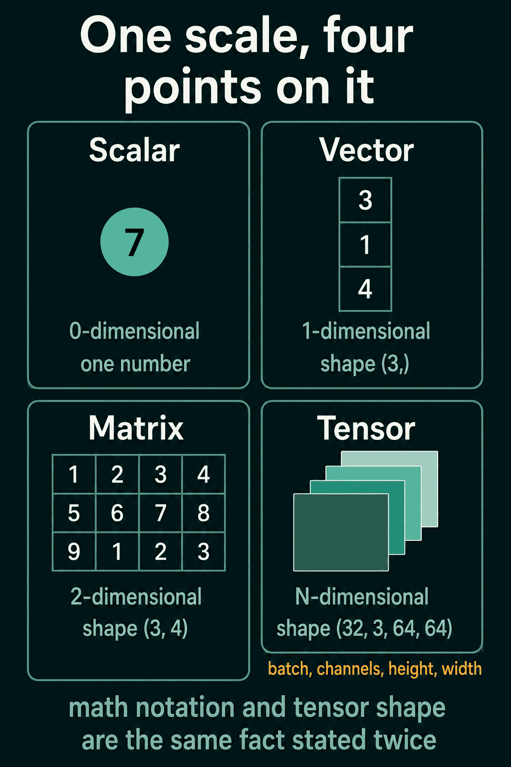
In code, the math and the tensor shape say the same thing. $A \in \mathbb{R}^{500 \times 4}$ is A.shape == (500, 4), $A_{ij}$ is A[i, j], A[i] is the whole $i$-th row and A[:, j] is the whole $j$-th column. Python counts from 0, so the first row is A[0].
1import torch
2
3s = torch.tensor(0.001)                      # scalar
4x = torch.tensor([1.0, 2.0, 3.0])            # vector in R^3
5A = torch.tensor([[1.0, 2.0, 3.0],
6                  [4.0, 5.0, 6.0]])          # matrix in R^(2x3)
7
8print(s.shape, x.shape, A.shape)
9print(A[1, 2])      # row 1, column 2 (counting from 0)
10print(A[1])         # the whole row 1
11print(A[:, 2]) # the whole column 21torch.Size([]) torch.Size([3]) torch.Size([2, 3])
2tensor(6.)
3tensor([4., 5., 6.])
4tensor([3., 6.])Adding and scaling vectors
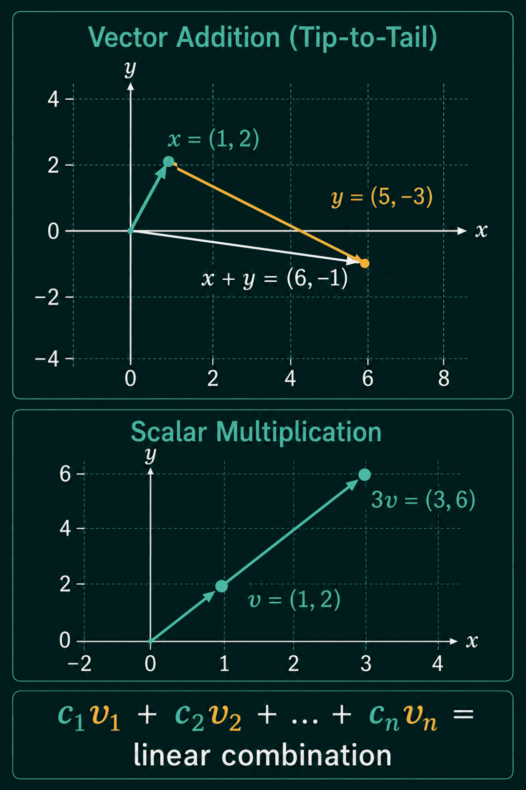
Addition goes entry by entry: line up the two vectors and add matching positions.
$$(\mathbf{x} + \mathbf{y})_i = x_i + y_i$$
So $(1, 2) + (5, -3) = (6, -1)$. Both vectors have to be the same length, since a leftover entry would have nothing to pair with.
Scaling multiplies every entry by the same number $c$:
$$(c\mathbf{x})_i = c,x_i$$
So $3(1, 2) = (3, 6)$, and $-1(1, 2) = (-1, -2)$ is the same length pointing the other way.
Combining the two gives a linear combination: scale a few vectors and add the results.
$$c_1\mathbf{v}_1 + c_2\mathbf{v}_2 + \cdots + c_n\mathbf{v}_n$$
The $c_i$ are the coefficients. $2(1, 0) + 3(0, 1) = (2, 3)$ is one.
In PyTorch both are plain arithmetic on tensors of the same shape:
1import torch
2
3x = torch.tensor([1.0, 2.0])
4y = torch.tensor([5.0, -3.0])
5
6print(x + y)          # entry by entry
7print(3 * x)          # scale every entry
8
9e1 = torch.tensor([1.0, 0.0])
10e2 = torch.tensor([0.0, 1.0])
11print(2 * e1 + 3 * e2) # a linear combination1tensor([ 6., -1.])
2tensor([3., 6.])
3tensor([2., 3.])The transpose
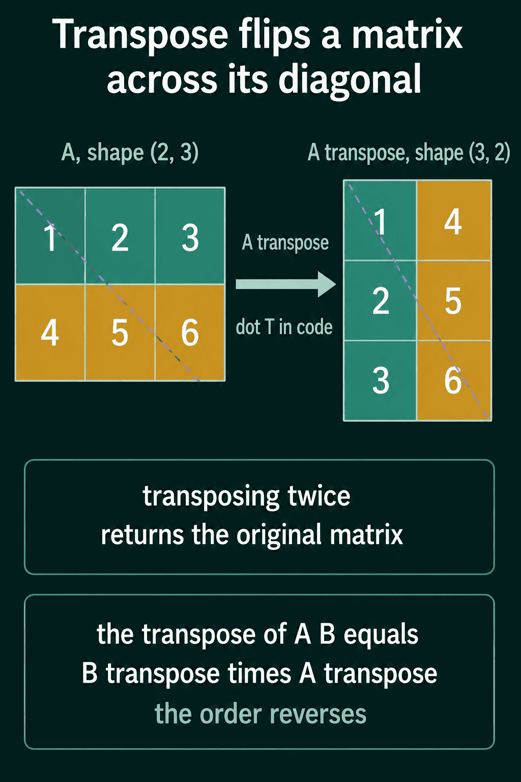
The transpose of a matrix $A$, written $A^\top$, flips it across its diagonal so that row $i$ becomes column $i$. A matrix of shape $(m, n)$ becomes $(n, m)$:
$$\begin{bmatrix} 1 & 2 & 3 \ 4 & 5 & 6 \end{bmatrix}^\top = \begin{bmatrix} 1 & 4 \ 2 & 5 \ 3 & 6 \end{bmatrix}$$
A vector transposes too: a column becomes a row. That is why formulas write $\mathbf{w}^\top \mathbf{x}$, where the $\top$ lines the shapes up so the multiplication is defined.
Two properties come up often. Transposing twice gives the original back, $(A^\top)^\top = A$. And for a matrix product $AB$ (written A @ B in PyTorch), the transpose reverses the order:
$$(AB)^\top = B^\top A^\top$$
1import torch
2
3A = torch.tensor([[1.0, 2.0, 3.0],
4                  [4.0, 5.0, 6.0]])
5B = torch.tensor([[1.0, 0.0],
6                  [2.0, 1.0],
7                  [0.0, 3.0]])
8
9print(A.T)
10print(A.T.shape)
11print(torch.equal(A.T.T, A))                 # transposing twice gives A back
12print(torch.equal((A @ B).T, B.T @ A.T)) # the order reverses1tensor([[1., 4.],
2 [2., 5.],
3 [3., 6.]])
4torch.Size([3, 2])
5True
6TrueThe transpose shows up in gradient formulas and whenever two matrices need their dimensions lined up before they can be multiplied.
Identity, diagonal and symmetric matrices
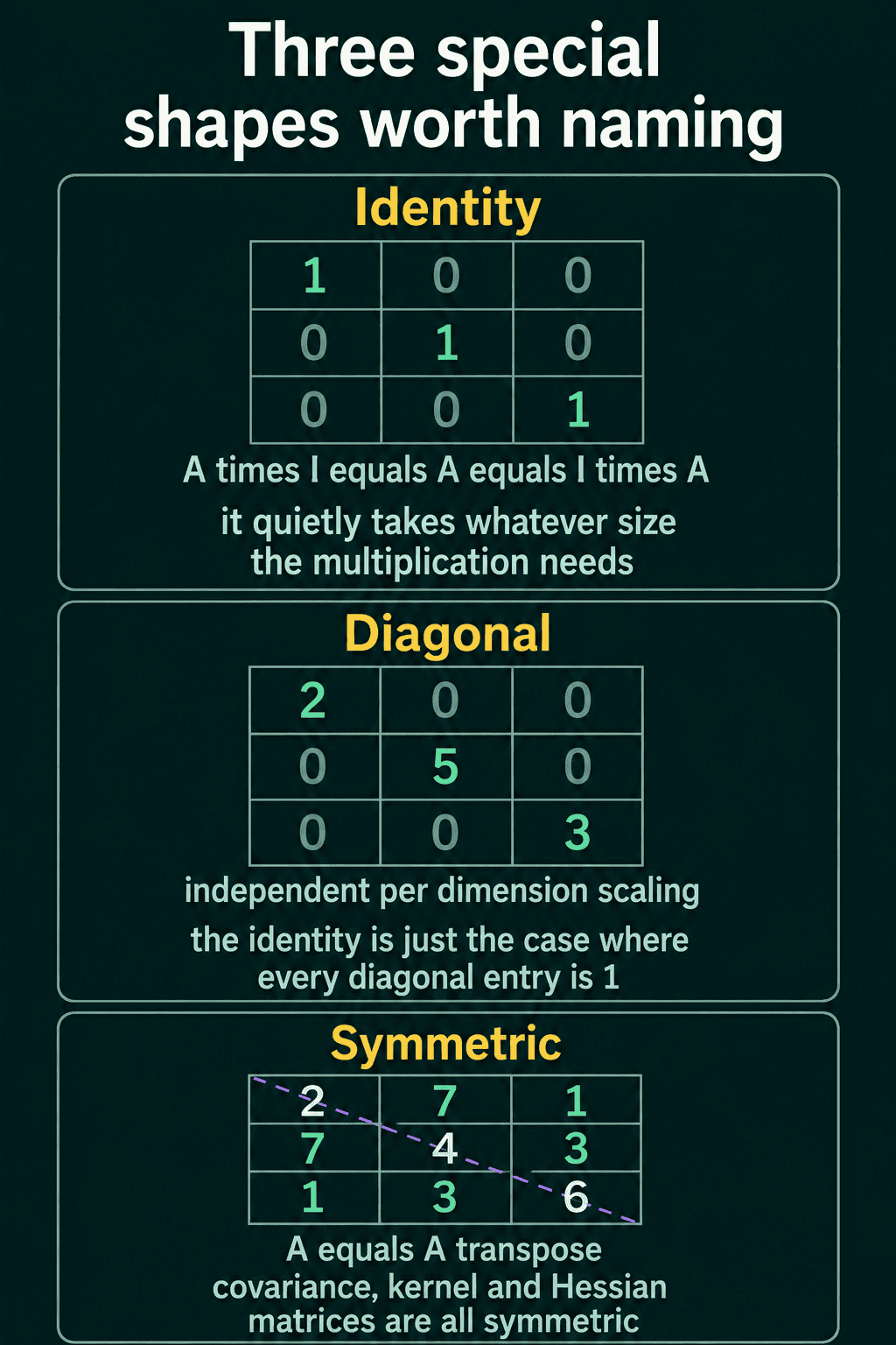
Three matrix patterns come up often enough to have names.
The identity matrix $I$ is square, with 1s down the diagonal and 0s elsewhere. Multiplying by it changes nothing:
$$AI = A = IA$$
Its size depends on the multiplication. If $A$ is $3 \times 5$, then $AI = A$ needs a $5 \times 5$ identity and $IA = A$ needs a $3 \times 3$ one.
A diagonal matrix, $\text{diag}(d_1, \ldots, d_n)$, has any values down the diagonal and 0s elsewhere. The identity is the case where every $d_i = 1$. Multiplying a vector by a diagonal matrix scales each entry by its own number, which is how a diagonal covariance matrix treats each dimension as unrelated to the others, and how a normalization layer applies a learned scale per channel.
A symmetric matrix satisfies $A = A^\top$, so flipping it across the diagonal gives the same matrix. Covariance matrices are symmetric.
1import torch
2
3A = torch.tensor([[1.0, 2.0, 3.0, 4.0, 5.0],
4                  [6.0, 7.0, 8.0, 9.0, 10.0],
5                  [11.0, 12.0, 13.0, 14.0, 15.0]])   # shape (3, 5)
6
7print(torch.equal(A @ torch.eye(5), A))   # A I = A needs a 5x5 identity
8print(torch.equal(torch.eye(3) @ A, A))   # I A = A needs a 3x3 identity
9
10D = torch.diag(torch.tensor([2.0, 5.0, 3.0]))
11print(D)
12print(D @ torch.tensor([1.0, 1.0, 1.0]))  # scales each entry separately
13
14S = torch.tensor([[2.0, 7.0, 1.0],
15                  [7.0, 4.0, 3.0],
16                  [1.0, 3.0, 6.0]])
17print(torch.equal(S, S.T)) # symmetric1True
2True
3tensor([[2., 0., 0.],
4 [0., 5., 0.],
5 [0., 0., 3.]])
6tensor([2., 5., 3.])
7TrueIf a shape check fails, print .shape on both sides before anything else, since most of these errors are a missing transpose or rows and columns swapped.
Common mistakes
- Swapping rows and columns. $\mathbb{R}^{m \times n}$ and
shape == (m, n)both put rows first. - Off-by-one indexing. Math usually counts from 1 and Python from 0, so $x_1$ is
x[0]. - Adding vectors of different lengths. Entry-by-entry addition needs matching shapes.
- Forgetting the order flip. $(AB)^\top$ is $B^\top A^\top$, not $A^\top B^\top$.
Related math
Span, basis and linear independence build on linear combinations: which points a set of vectors can reach, and how few vectors it takes. They are covered in span, basis and linear independence explained. The shape notation itself, $\in \mathbb{R}^{m \times n}$, is in how to read the math notation in ML papers.
QuiddityML teaches each of these as its own concept in the linear algebra part of the Math track, and the exercises include pulling a sample row and a feature column out of a dataset tensor, picking the code that computes $(AB)^\top$ without multiplying $A$ and $B$ first, and building a diagonal matrix from a vector.