By Sagi Shaier · 11 October 2026 · 6 min read

Partial derivatives and gradients explained

How to take the derivative of a function with several inputs one input at a time, how those derivatives stack into the gradient, and why stepping against the gradient lowers a loss fastest, with worked examples and PyTorch checks.

A partial derivative is the slope of a function of several inputs along one input, with every other input held fixed. Stacking one partial derivative per input into a vector gives the gradient, and the gradient of the loss with respect to a model's weights is what gradient descent uses to decide how to change every weight at once.

Why one derivative is not enough

An ordinary derivative measures how the output of $f(x)$ changes as its single input $x$ moves: it is the slope of the curve at that point. A neural network's loss depends on every weight and bias in the network at the same time, often millions of numbers. The question becomes how the loss changes when one of those numbers moves and the rest stay put, and that question has one answer per weight.

The partial derivative

To find how $f$ changes with respect to one variable, hold every other variable fixed and differentiate as usual, treating the others as constants.

For a function $f(x, y)$ of two inputs, the partial derivative with respect to $x$ is written $\frac{\partial f}{\partial x}$. The curly $\partial$ in place of a straight $d$ signals that the function has other inputs and they are being held fixed. With $h$ as a small step in $x$, the definition is the same limit as an ordinary derivative, with only $x$ moving:

$$\frac{\partial f}{\partial x} = \lim_{h \to 0} \frac{f(x+h, y) - f(x, y)}{h}$$

As $h$ shrinks toward 0, this fraction approaches the slope of $f$ in the $x$ direction at the point $(x, y)$, while $y$ stays where it is.

Worked example

Let $f(x, y) = x^2 y + y^3$.

For $\frac{\partial f}{\partial x}$, treat $y$ as a constant. The term $x^2 y$ is then a constant $y$ times $x^2$, and the power rule ($\frac{d}{dx} x^n = n x^{n-1}$) gives $2xy$. The term $y^3$ has no $x$ in it, so it is a constant as far as $x$ is concerned, and its derivative is 0:

$$\frac{\partial f}{\partial x} = 2xy$$

For $\frac{\partial f}{\partial y}$, treat $x$ as the constant instead. The term $x^2 y$ is a constant $x^2$ times $y$, which gives $x^2$, and $y^3$ gives $3y^2$:

$$\frac{\partial f}{\partial y} = x^2 + 3y^2$$

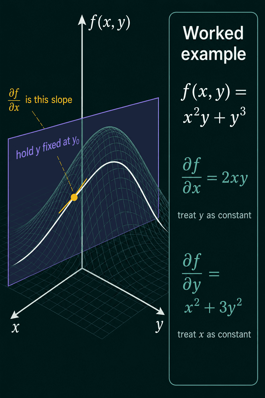
A 3D surface f(x, y) cut by a vertical plane that holds y fixed at y0, where the slope of the curve where the plane meets the surface is the partial derivative with respect to x, next to the worked example f(x, y) = x squared y plus y cubed with partial f over partial x = 2xy (treat y as constant) and partial f over partial y = x squared plus 3y squared (treat x as constant)

Holding $y$ fixed slices the surface along one curve, and $\frac{\partial f}{\partial x}$ is the slope of that curve. Moving one input at a time in code gives the same numbers. At $(x, y) = (2, 1)$ the formulas give $2 \cdot 2 \cdot 1 = 4$ and $2^2 + 3 \cdot 1^2 = 7$:

1def f(x, y):
2    return x**2 * y + y**3
3 
4x, y, h = 2.0, 1.0, 1e-6
5df_dx = (f(x + h, y) - f(x, y)) / h   # only x moves
6df_dy = (f(x, y + h) - f(x, y)) / h   # only y moves
7print(round(df_dx, 4), 2 * x * y)
8print(round(df_dy, 4), x**2 + 3 * y**2)

14.0 4.0
27.0 7.0

A function of $n$ variables has $n$ partial derivatives, one per input.

The gradient

The gradient collects all the partial derivatives of a function into one vector. The symbol $\nabla$ (read "nabla") means "the gradient of," and for two inputs:

$$\nabla f(x, y) = \begin{bmatrix} \dfrac{\partial f}{\partial x} \\[10pt] \dfrac{\partial f}{\partial y} \end{bmatrix}$$

For a function of $n$ variables, $\nabla f$ is a vector of $n$ numbers. For the worked example at $(2, 1)$, the gradient is $(4, 7)$.

The gradient has a geometric meaning: it points in the direction where $f$ increases fastest, and its length is how steep that increase is. Gradient descent makes a loss smaller as quickly as possible by moving the weights in the opposite direction, $-\nabla f$.

Why the gradient points uphill

The reason comes from the directional derivative, the rate at which $f$ changes when the input steps in a chosen direction. For a direction given by a unit vector $\mathbf{u}$ (a vector of length 1), that rate is the dot product of the gradient with $\mathbf{u}$:

$$D_{\mathbf{u}} f(x) = \nabla f(x) \cdot \mathbf{u}$$

A dot product can also be written with the angle $\theta$ between the two vectors, as the product of their lengths times $\cos\theta$. Since $\mathbf{u}$ has length 1, with $\|\nabla f\|$ for the length of the gradient:

$$D_{\mathbf{u}} f(x) = \|\nabla f\| \cos\theta$$

Four facts follow from this one line:

The rate is largest at $\theta = 0$, when $\mathbf{u}$ points along the gradient, so $f$ climbs fastest in the gradient's direction.
That largest rate is $\|\nabla f\|$, so the gradient's length measures how steep the climb is.
The rate is 0 at $\theta = 90°$, so a step perpendicular to the gradient leaves $f$ unchanged to first order.
The rate is most negative at $\theta = 180°$, which is why descent steps along $-\nabla f$.

Worked example: the gradient of a sum of squares

Let $f(x) = \|x\|^2 = \sum_i x_i^2$, the sum of the squares of a vector's entries. This is the shape of a simple loss, such as a squared error. For one entry $x_i$, every other entry is held fixed and contributes 0, and the power rule gives $\frac{\partial f}{\partial x_i} = 2x_i$. Every entry works the same way, so the whole gradient is

$$\nabla f(x) = 2x$$

which doubles every entry of $x$. At the point $(2, 2)$ the gradient is $(4, 4)$, pointing straight away from the origin, where $f$ is smallest.

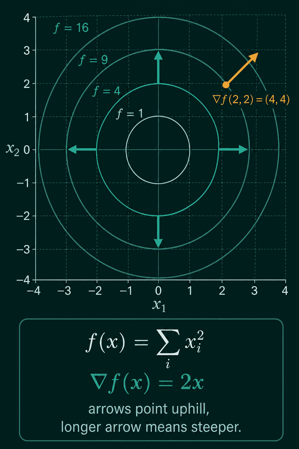
Circles of constant f = 1, 4, 9, 16 around the origin for f(x) = sum of x_i squared, with gradient arrows pointing outward and the gradient at (2, 2) equal to (4, 4), where arrows point uphill and a longer arrow means steeper

The directional derivative at $(2, 2)$ can be checked in each of the three directions above:

1import torch
2 
3x = torch.tensor([2.0, 2.0])
4grad = 2 * x                           # gradient of f(x) = sum of x_i squared
5print(grad, grad.norm())
6 
7for name, u in [("along the gradient", grad / grad.norm()),
8                ("perpendicular", torch.tensor([1.0, -1.0]) / 2**0.5),
9                ("against the gradient", -grad / grad.norm())]:
10    print(name, round((grad @ u).item(), 4))

1tensor([4., 4.]) tensor(5.6569)
2along the gradient 5.6569
3perpendicular 0.0
4against the gradient -5.6569

Along the gradient the rate equals the gradient's length, $\sqrt{4^2 + 4^2} \approx 5.6569$. Perpendicular to it the rate is 0, and against it the rate is the most negative value possible.

PyTorch can compute the same gradient automatically, which is how gradients of real losses get computed in practice:

1import torch
2 
3x = torch.tensor([1.0, 2.0, 3.0], requires_grad=True)
4f = (x**2).sum()
5f.backward()
6print(x.grad)
7print(2 * x.detach())

1tensor([2., 4., 6.])
2tensor([2., 4., 6.])

Common mistakes

Dropping a term that only looks constant. In $\frac{\partial f}{\partial y}$ of $x^2 y + y^3$, the $x^2 y$ term still depends on $y$ and contributes $x^2$. Only terms with no $y$ in them become 0.
Treating a held-fixed variable as zero. Holding $y$ fixed means it keeps its value, so $\frac{\partial f}{\partial x} = 2xy$ still has $y$ in it.
Mixing up the gradient and the step. The gradient points uphill. A training step that lowers the loss moves along $-\nabla f$.
Using a direction that is not unit length. $\nabla f \cdot \mathbf{u}$ is the rate of change only when $\mathbf{u}$ has length 1. Divide by the vector's length first.

A partial derivative is an ordinary derivative with the other inputs frozen. The single-input version, built from a limit, is in derivatives for machine learning. The dot product that gives the directional derivative is in the dot product explained, and the vector length $\|x\|$ is in vector norms and distances.

QuiddityML teaches partial derivatives and gradients as two concepts in the calculus part of the Math track, with exercises that find $\frac{\partial f}{\partial y}$ for a two-variable function and pick the assertion that checks a gradient of $[2, 4, 6]$. The last one is writing gradient(x) for $\|x\|^2$ from scratch.