By Sagi Shaier · 13 October 2026 · 7 min read

Taylor series for machine learning: linearization and why gradient descent works

How to approximate a function near a point with its gradient and Hessian, how far you can trust that approximation, and what it says about why a small gradient descent step lowers the loss, with worked numbers and PyTorch code.

A Taylor series rewrites a function near a point as a sum of simple terms built from its derivatives at that point. Keeping only the first one or two terms gives an approximation that is easy to compute and accurate for small moves. Gradient descent relies on that approximation each time it takes a step.

The idea in one dimension

Zoom in close enough on a smooth curve and it looks almost straight. The slope of that nearly straight piece is the derivative, written $f'(a)$ at a point $a$. So to estimate the function a small distance $h$ away from $a$, start at $f(a)$ and move along the slope:

$$f(a + h) \approx f(a) + f'(a)\, h$$

Take $f(x) = x^2$ at $a = 3$. Here $f(3) = 9$ and $f'(3) = 6$. For $h = 0.1$ the estimate is $9 + 6 \cdot 0.1 = 9.6$. The true value is $3.1^2 = 9.61$, so the straight line misses by $0.01$. The miss comes from the curve bending away from the line, and it grows as $h$ grows.

Linearization with many inputs

A loss depends on many parameters, so the step is a vector $\Delta$ with one entry per parameter. The slope becomes the gradient $\nabla f(x)$, the vector of partial derivatives of $f$ at the point $x$. A partial derivative is the slope along one input while the others stay fixed. Moving along the slope in the direction $\Delta$ means taking the dot product of the gradient with the step:

$$f(x+\Delta) \approx f(x) + \nabla f(x) \cdot \Delta$$

To estimate the function a small step $\Delta$ away from $x$, start at $f(x)$ and add the gradient dotted with the step. This is called linearization, and it is the first-order Taylor approximation of $f$ around $x$. It is first-order because it uses only first derivatives.

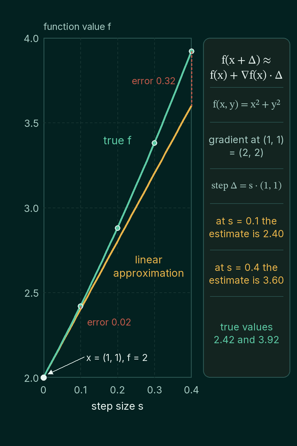
Take $f(x, y) = x^2 + y^2$ at the point $(1, 1)$, where $f = 2$. The gradient is $(2x, 2y) = (2, 2)$. For the step $\Delta = (0.1, 0.1)$:

$$f(x) + \nabla f(x) \cdot \Delta = 2 + 2 \cdot 0.1 + 2 \cdot 0.1 = 2.40$$

The true value is $f(1.1, 1.1) = 1.21 + 1.21 = 2.42$, so the estimate is off by $0.02$. Make the step four times larger, $\Delta = (0.4, 0.4)$, and the estimate is $2 + 0.8 + 0.8 = 3.60$ while the true value is $1.4^2 + 1.4^2 = 3.92$. The error grew from $0.02$ to $0.32$, sixteen times larger for a step four times larger.

Why gradient descent works

A gradient descent step moves the parameters against the gradient: $\Delta = -\eta \nabla f(x)$, where $\eta$ is a small positive number called the learning rate. Put that step into the linearization:

$$f(x - \eta \nabla f(x)) \approx f(x) - \eta\, \nabla f(x) \cdot \nabla f(x)$$

The dot product of a vector with itself is the sum of its squared entries, so $\nabla f(x) \cdot \nabla f(x)$ is positive whenever the gradient is not zero. The approximation therefore says the loss goes down. That prediction holds only while the linearization is accurate, which is why the step has to be small.

At $(1, 1)$ with $\eta = 0.1$, the gradient is $(2, 2)$, so the step is $(-0.2, -0.2)$. The linearization predicts $2 - 0.1 \cdot (4 + 4) = 1.20$. The true value after the step is $0.8^2 + 0.8^2 = 1.28$. The loss did go down, by a little less than the straight line promised, because the function curves.

1import torch
2 
3def f(p):
4    return (p ** 2).sum()                # f(x, y) = x^2 + y^2
5 
6x = torch.tensor([1.0, 1.0], requires_grad=True)
7lr = 0.1
8loss = f(x)
9grad, = torch.autograd.grad(loss, x)
10step = -lr * grad                        # gradient descent step
11predicted = loss - lr * grad @ grad      # linear prediction of the new loss
12print(f"{loss.item():.2f} {predicted.item():.2f} {f(x.detach() + step).item():.2f}")
13# 2.00 1.20 1.28

Adding curvature: the second-order term

The missing piece in every example so far is curvature. The Hessian $H(x)$ is the matrix of second partial derivatives of $f$, and it describes how the slope changes as you move. Adding one term built from it gives the second-order Taylor expansion:

$$f(x+\Delta) \approx f(x) + \nabla f(x) \cdot \Delta + \frac{1}{2} \Delta^T H(x) \Delta$$

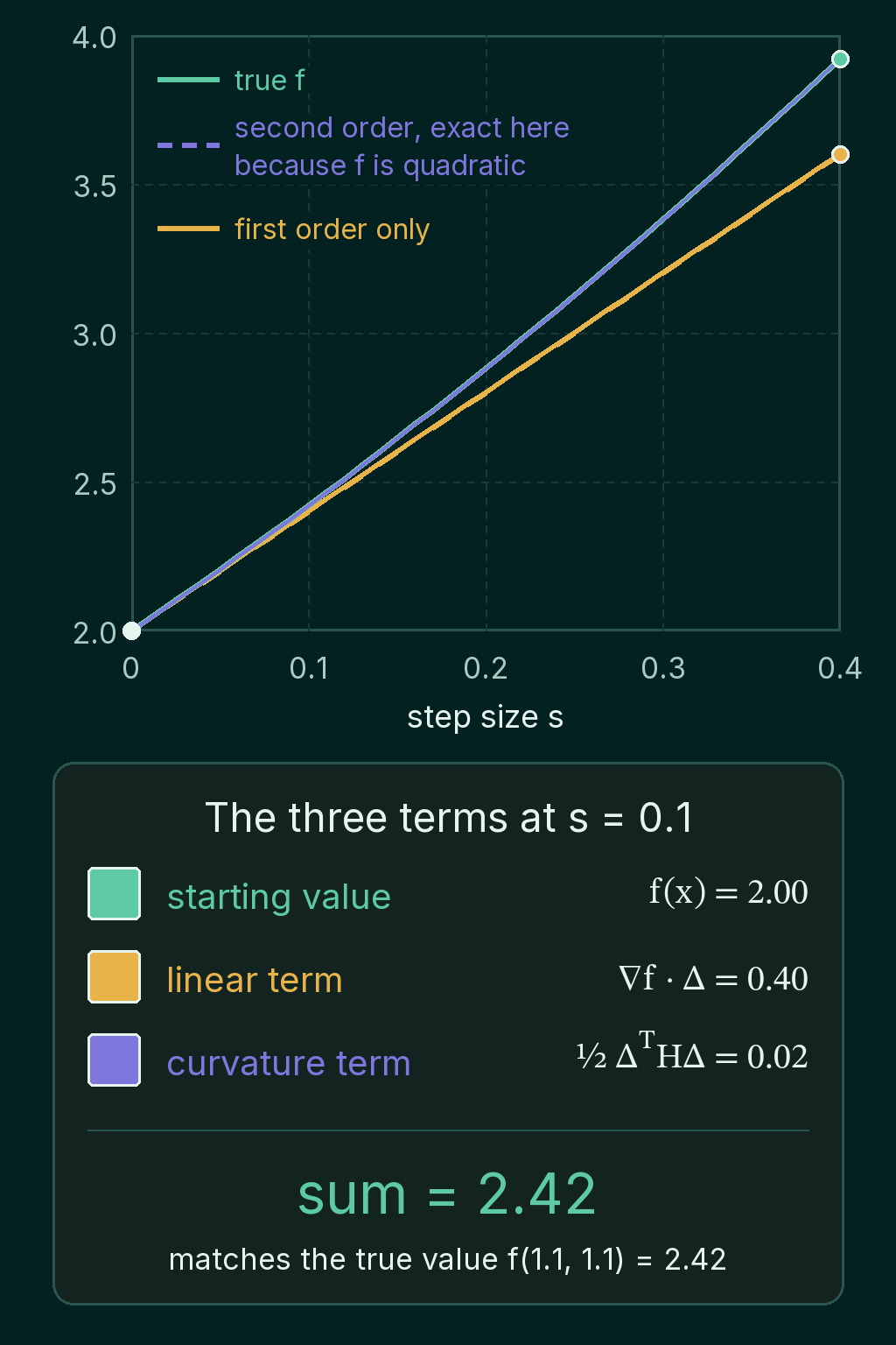
The three pieces are where you start, the linear correction, and a curvature correction. The last one, $\Delta^T H \Delta$, is a single number. First multiply the Hessian by the step to get the vector $H\Delta$. Then take the dot product of the step with that vector. It measures how much the slope itself changes over the course of the step.

For $f(x, y) = x^2 + y^2$ the Hessian is the same everywhere:

$$H = \begin{bmatrix} 2 & 0 \\ 0 & 2 \end{bmatrix}$$

With $\Delta = (0.1, 0.1)$, $H\Delta = (0.2, 0.2)$ and $\Delta \cdot H\Delta = 0.02 + 0.02 = 0.04$. Half of that is $0.02$. Adding it to the linear estimate gives $2.40 + 0.02 = 2.42$, exactly the true value. That is not luck: $f$ is a quadratic, so its third and higher derivatives are zero and the second-order expansion has nothing left to miss.

Where the one half comes from

The full Taylor series of a one-input function around a point $a$ keeps going, adding one more derivative and one more factorial each time:

$$f(x) = f(a) + f'(a)(x-a) + \frac{f''(a)}{2!}(x-a)^2 + \frac{f'''(a)}{3!}(x-a)^3 + \cdots$$

$n!$ is read "n factorial" and is the product $1 \cdot 2 \cdots n$, so $2! = 2$ and $3! = 6$. Cutting the sum after the first-derivative term gives linearization. Cutting it after the second-derivative term gives the second-order expansion, and the $1/2$ in front of $\Delta^T H \Delta$ is the $1/2!$ from that term. With many inputs, $f''(a)$ becomes the Hessian and $(x - a)^2$ becomes $\Delta^T H \Delta$.

For a function that is not a polynomial, each extra term shrinks the error near the point. Take $f(x) = e^x$ around $a = 0$. Every derivative of $e^x$ is $e^x$, which is $1$ at $0$, so the first terms are $1 + x + x^2/2$:

At $x = 0.1$ the second-order estimate is off by less than $0.0002$. At $x = 1.0$ it is off by more than $0.2$. Truncating the series leaves an error term, and that error grows as the point moves away from $a$.

Computing both approximations in PyTorch

1import torch
2from torch.autograd.functional import hessian
3 
4def f(p):
5    return (p ** 2).sum()            # f(x, y) = x^2 + y^2
6 
7x = torch.tensor([1.0, 1.0], requires_grad=True)
8fx = f(x)
9grad, = torch.autograd.grad(fx, x)
10H = hessian(f, x.detach())
11 
12for s in [0.1, 0.4]:
13    delta = torch.tensor([s, s])
14    first = fx + grad @ delta
15    second = first + 0.5 * delta @ H @ delta
16    true = f(x.detach() + delta)
17    print(f"s={s}: first {first.item():.2f}  second {second.item():.2f}  true {true.item():.2f}")
18# s=0.1: first 2.40  second 2.42  true 2.42
19# s=0.4: first 3.60  second 3.92  true 3.92

Swap in your own f to see how fast each approximation drifts. For a function that is not quadratic, the second-order column usually drifts away from the true column as s grows.

When to use it, and common mistakes

Linearization is the reasoning behind a gradient step: it predicts that a small move against the gradient lowers the loss. The second-order expansion says how wrong that prediction is, and the curvature term is what tells you a step was too large. Both are local tools, accurate near the point where the derivatives were taken.

• Trusting the linear estimate for large steps. The error grows faster than the step. In the example above, four times the step gave sixteen times the error.
• Dropping the one half. The curvature term is $(1/2) \Delta^T H \Delta$. Without the $1/2$ the example would give $2.44$ instead of $2.42$.
• Reading $\Delta^T H \Delta$ as a matrix. It is a single number: the step dotted with the Hessian times the step.
• Building the Hessian for a large model. A model with $n$ parameters has an $n \times n$ Hessian, so one million parameters would mean a trillion entries. The second-order expansion is a tool for reasoning about steps and small problems, not something computed in full for a large network.

Related concepts

The Hessian matrix supplies the curvature term, and its eigenvalues say whether the function curves up or down in each direction. Convex functions are the ones whose curvature term is never negative, so the straight-line estimate never comes out above the true value. Critical points are where the gradient term vanishes. There the curvature term decides whether the point is a minimum, a maximum or a saddle.

QuiddityML teaches Taylor series and linearization as their own concept in the Math track. The exercises on it include turning the second-order formula into code, picking the arguments a taylor_approx function needs and writing that function from scratch in PyTorch.