By Sagi Shaier · 4 November 2026 · 9 min read

Encoder-decoder (seq2seq) models explained

What the encoder and the decoder each compute, how one context vector connects them in PyTorch code, and why that single vector struggles with long inputs.

An encoder-decoder model is two networks joined together. The encoder reads an input sequence and turns it into vectors of numbers, and the decoder turns those vectors into an output sequence one token at a time. It is the classic way to build sequence-to-sequence (seq2seq) models for tasks such as translation, where the input and the output are both sequences and their lengths can differ. In text, a token is a whole word or a piece of a word.

What kind of task needs seq2seq?

Many tasks have a fixed relation between input and output length:

• Many-to-one: a whole sentence goes in and one label comes out, as in sentiment classification.
• Many-to-many with the same length: one label comes out per input token, as in tagging each word with its part of speech.
• One-to-many: one input produces a sequence, as in writing a caption for an image.

Translation fits none of these. The English "thank you very much" has four words and the German "danke schön" has two, and the word order can change between languages too. Sequence-to-sequence is the many-to-many pattern where the input and output lengths can differ. The model reads a source sequence and then produces a target sequence.

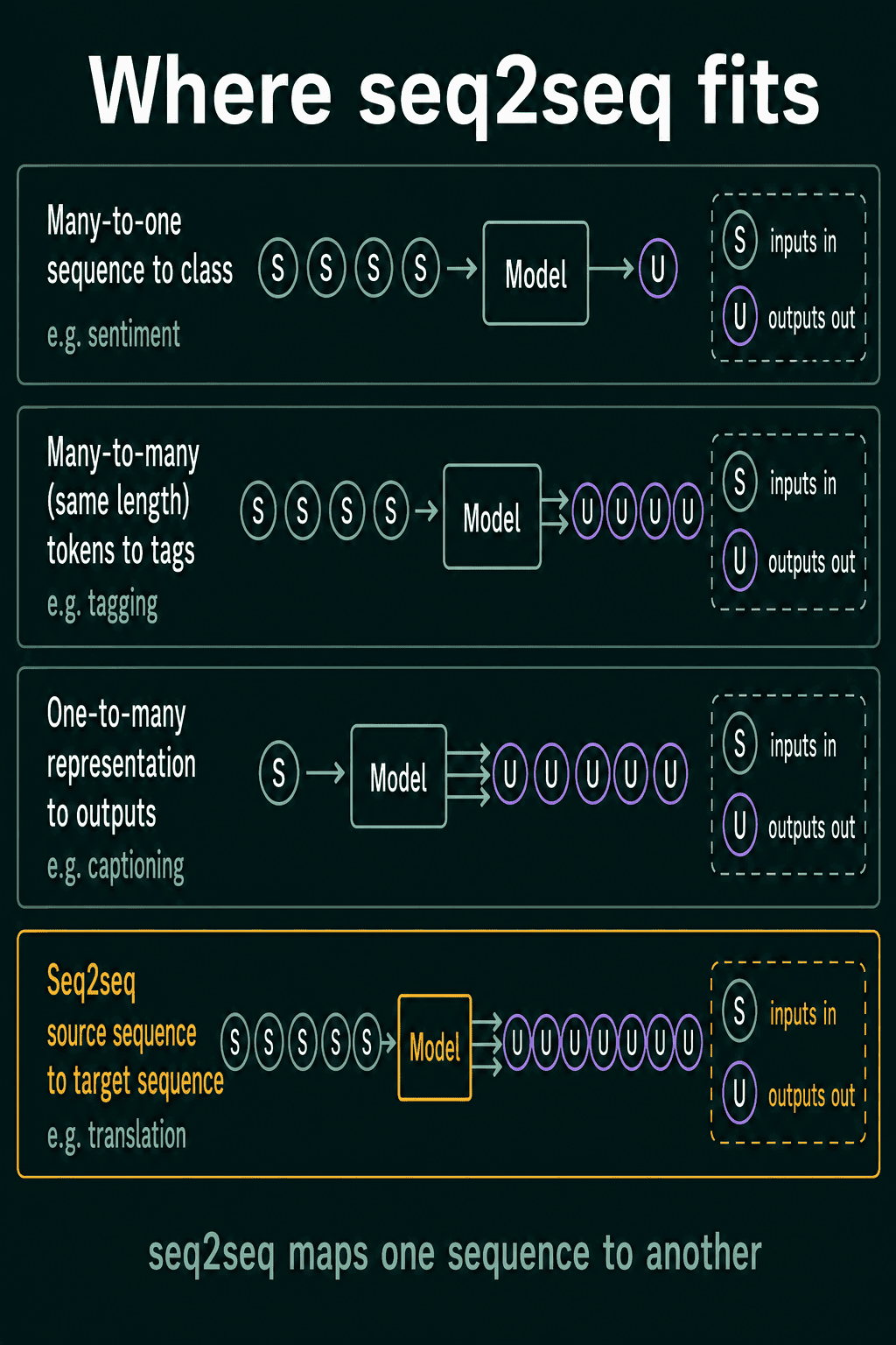
Encoder-decoder is one way to build this shape with recurrent networks. A decoder-only model, which only generates text, can also translate when the source text is placed at the start of its input.

What an encoder is

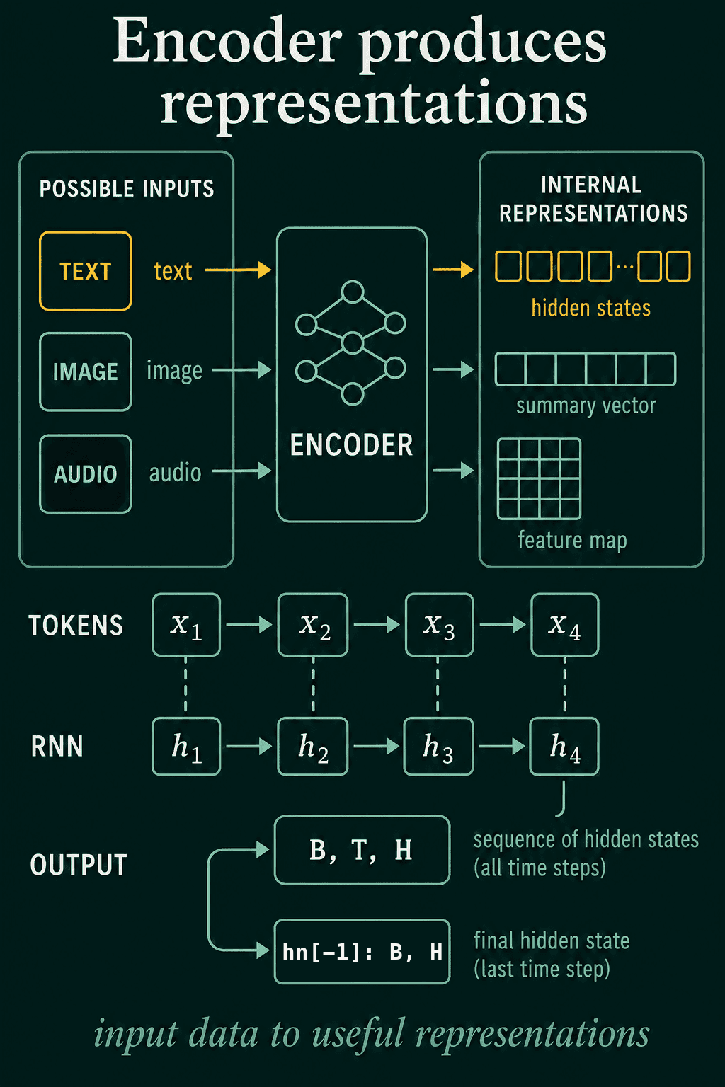
An encoder is a model, or part of a model, that reads input data and turns it into internal representations. These representations are vectors of numbers that describe the input. The input can be a sentence, an image or audio. The encoder's output is usually not the final answer. It is something another component reads, such as a classifier head, a tagger or a decoder.

The word encoder names the job the network does. An encoder can be a recurrent network, an LSTM or a GRU, and it can also be a convolutional network or a transformer. For an image, the encoder often returns a grid of vectors called a feature map.

In the diagram below, B is the batch size (how many sequences go in together), T is the number of steps and H is the hidden size.

What an RNN encoder returns

Here the encoder is a recurrent neural network (RNN). It reads the source tokens $\mathbf{x}_1, \ldots, \mathbf{x}_S$ one at a time, where $S$ is the source length and each $\mathbf{x}_t$ is the vector for one token. At each step it updates its hidden state $\mathbf{h}_t$ from the current input and the previous hidden state:

$$\mathbf{h}_t = f(\mathbf{x}_t, \mathbf{h}_{t-1})$$

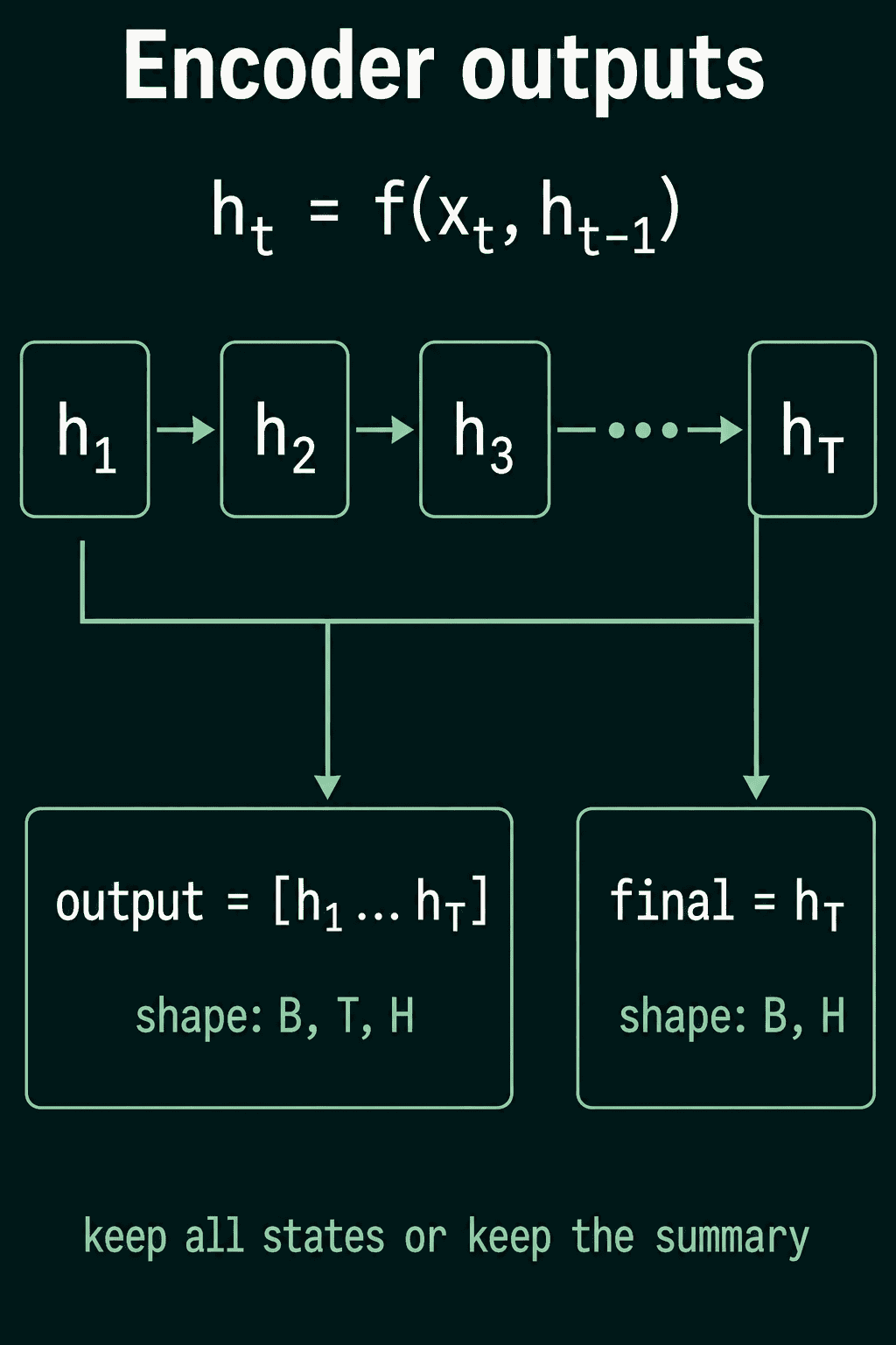
Here $f$ is the ordinary RNN update, $\tanh(\mathbf{W}_h \mathbf{h}_{t-1} + \mathbf{W}_x \mathbf{x}_t + \mathbf{b})$, with learned matrices $\mathbf{W}_h$ and $\mathbf{W}_x$ and a learned bias $\mathbf{b}$. After the last source token, the encoder can return two things. The first is every hidden state, one per source token:

$$\texttt{output} = [\mathbf{h}_1, \mathbf{h}_2, \ldots, \mathbf{h}_S]$$

The second is the last hidden state alone, which has read the whole sequence:

$$\texttt{summary} = \mathbf{h}_S$$

The task decides which one to use. A classifier usually reads the summary. A tagger reads output, because it needs one vector per token. A basic decoder starts from the summary.

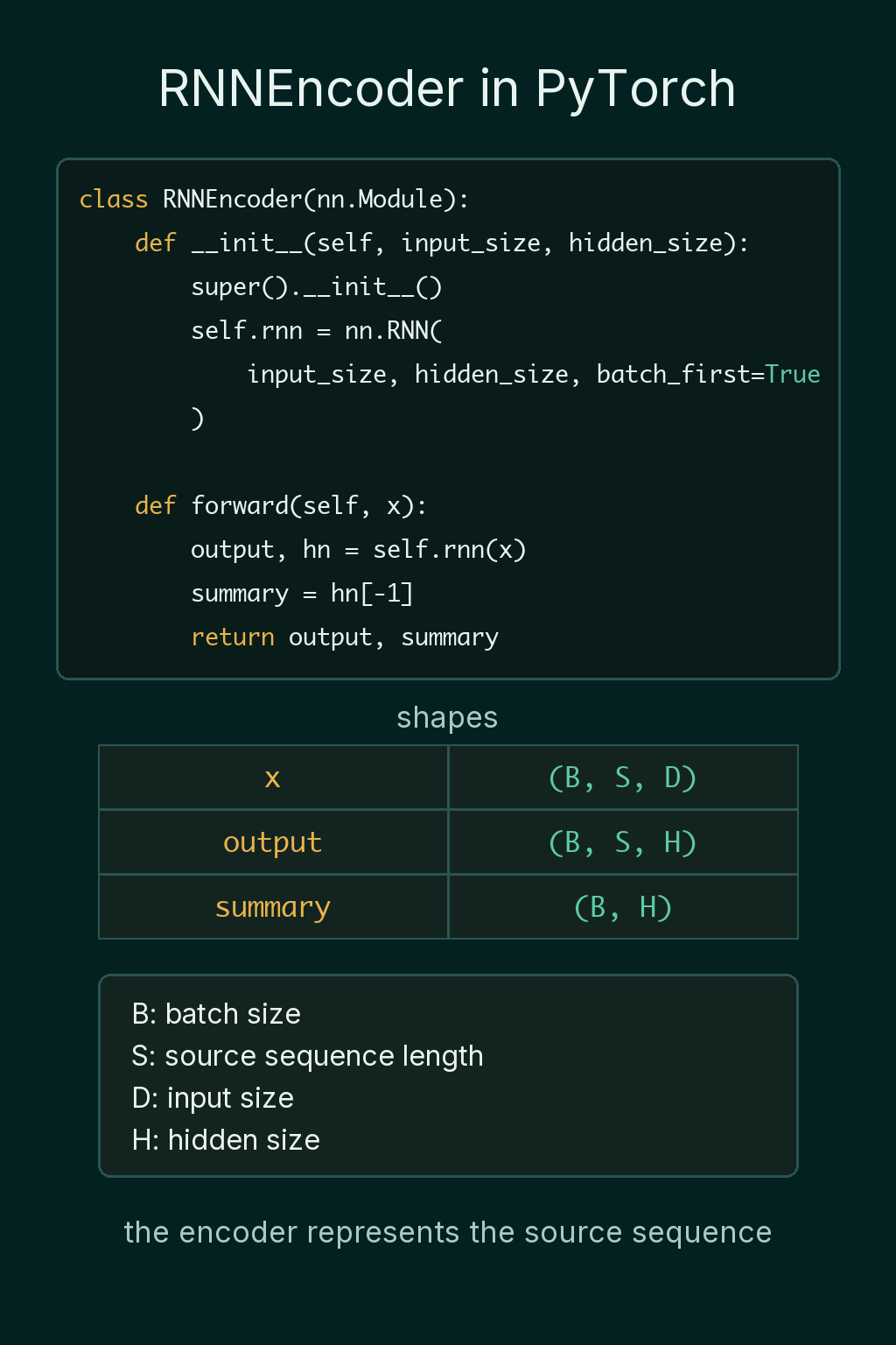
In PyTorch the encoder wraps one recurrent layer and returns both:

1import torch
2import torch.nn as nn
3 
4class RNNEncoder(nn.Module):
5    def __init__(self, input_size, hidden_size):
6        super().__init__()
7        self.rnn = nn.RNN(
8            input_size, hidden_size, batch_first=True
9        )
10 
11    def forward(self, x):
12        output, hn = self.rnn(x)
13        summary = hn[-1]
14        return output, summary
15 
16torch.manual_seed(0)
17encoder = RNNEncoder(input_size=32, hidden_size=128)
18x = torch.rand(4, 10, 32)  # 4 sentences, 10 tokens each, 32 numbers per token
19output, summary = encoder(x)
20print(output.shape)
21print(summary.shape)

1torch.Size([4, 10, 128])
2torch.Size([4, 128])

With batch_first=True, the input is laid out as (batch, source length, input size). output keeps one 128-number hidden state for each of the 10 tokens. hn has an extra first dimension that counts layers, and hn[-1] takes the last layer's final state, one vector per sentence. The encoder does not produce any target tokens by itself.

What a decoder is

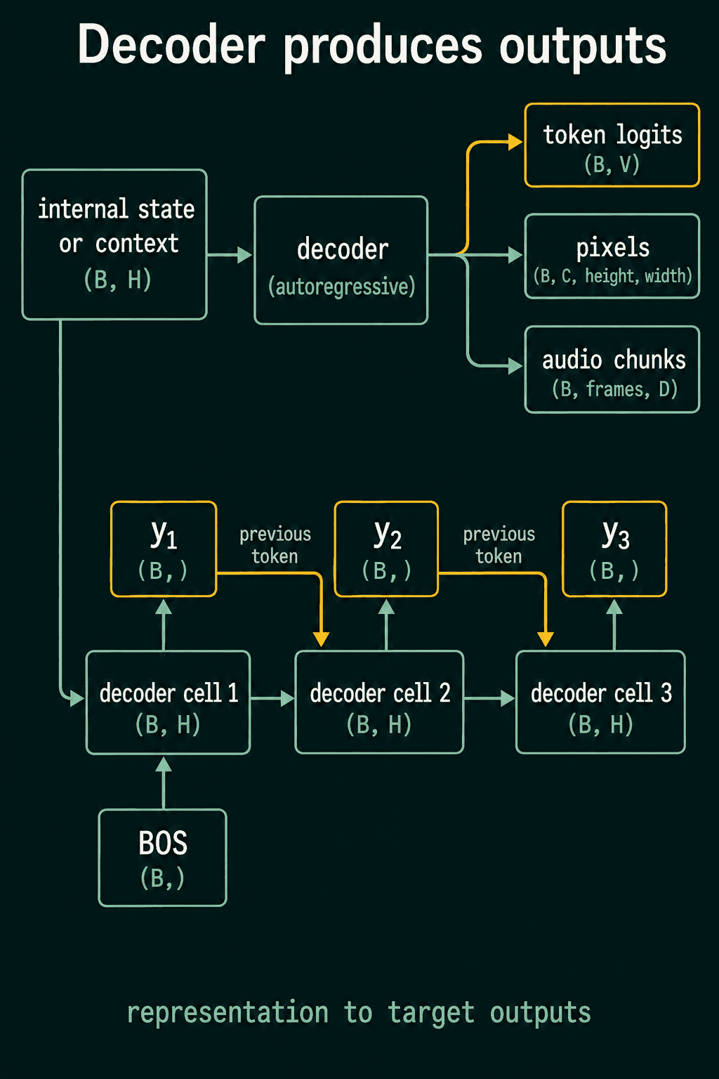
A decoder is a model, or part of a model, that turns an internal representation into outputs. What it outputs depends on the task. An image decoder can produce pixels and an audio decoder can produce chunks of a waveform. In text generation, the decoder produces logits one step at a time. Logits are one score for every token in the vocabulary.

The softmax function turns logits into probabilities that add up to 1. For example, logits of $[2.0, 1.0, 0.1]$ over a three-token vocabulary become probabilities of about $[0.659, 0.242, 0.099]$.

A text decoder needs a previous token at every step, including the first one. So the target side starts with a special start token, often written BOS for "beginning of sequence".

What the decoder computes at each step

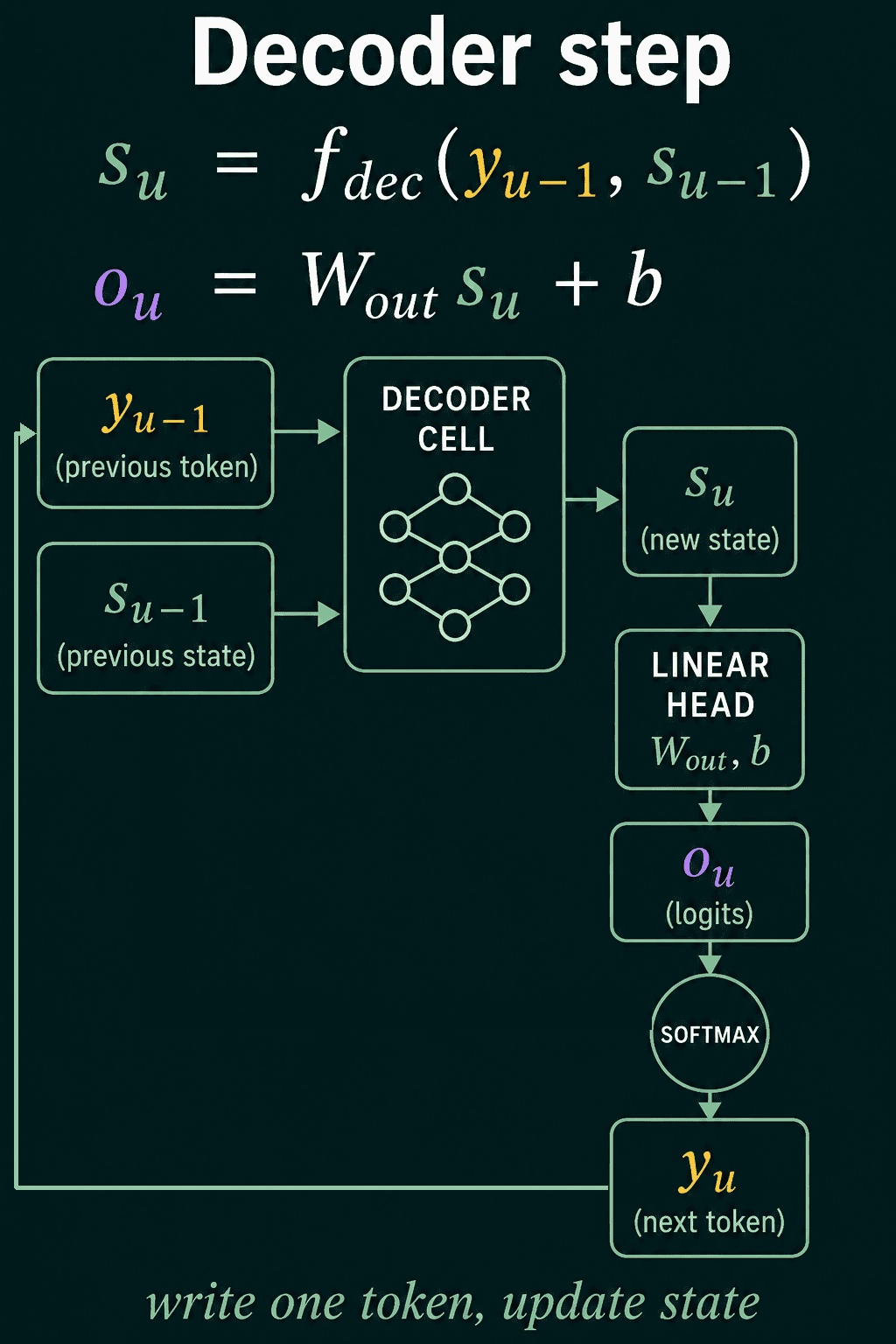
The decoder counts its own steps with $u$, so $y_u$ is the target token at step $u$. It keeps its own state $\mathbf{s}_u$, a different letter from the encoder's $\mathbf{h}_t$ to keep the two apart. At step $u$ it reads $\mathbf{y}_{u-1}$, the embedding of the previous target token (the vector that represents that token), together with its previous state $\mathbf{s}_{u-1}$:

$$\mathbf{s}_u = f_{\text{dec}}(\mathbf{y}_{u-1}, \mathbf{s}_{u-1})$$

A linear layer with weights $\mathbf{W}_{\text{out}}$ and bias $\mathbf{b}_{\text{out}}$, called the vocabulary head, maps the state to logits $\mathbf{o}_u$:

$$\mathbf{o}_u = \mathbf{W}_{\text{out}}\mathbf{s}_u + \mathbf{b}_{\text{out}}$$

Softmax turns those logits into a probability for every possible next token. $y_{<u}$ means all target tokens before step $u$, and the context is whatever the decoder started from:

$$P(y_u \mid y_{<u}, \text{context}) = \mathrm{softmax}(\mathbf{o}_u)$$

During training, the previous-token inputs usually come from the correct target sentence. During generation, the decoder feeds the token it chose at step $u$ back in as the previous token for step $u + 1$.

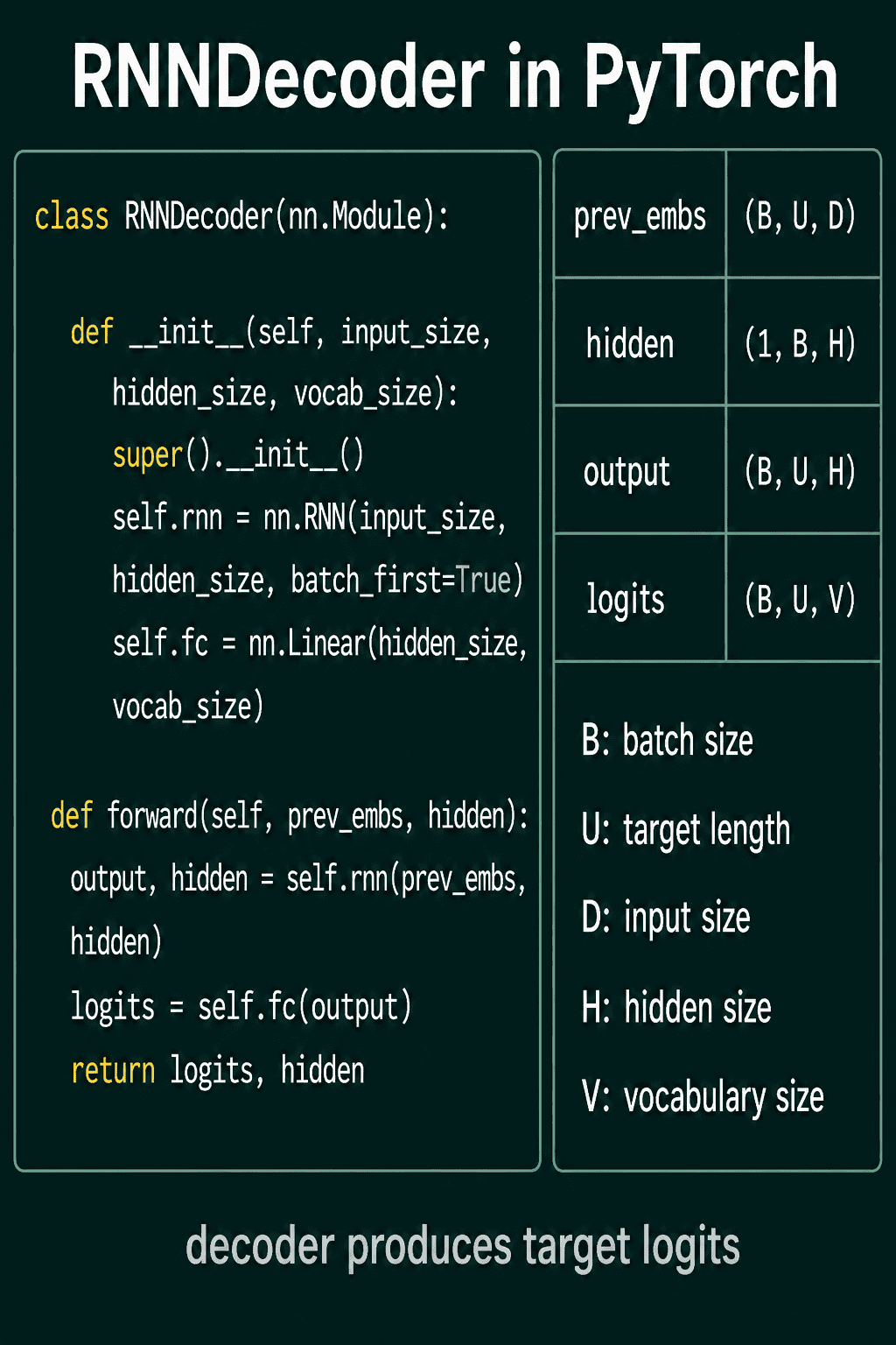
In PyTorch the decoder wraps one recurrent layer and one vocabulary head:

1class RNNDecoder(nn.Module):
2    def __init__(self, input_size, hidden_size, vocab_size):
3        super().__init__()
4        self.rnn = nn.RNN(
5            input_size, hidden_size, batch_first=True
6        )
7        self.fc = nn.Linear(hidden_size, vocab_size)
8 
9    def forward(self, prev_embs, hidden):
10        output, hidden = self.rnn(prev_embs, hidden)
11        logits = self.fc(output)
12        return logits, hidden
13 
14decoder = RNNDecoder(input_size=32, hidden_size=128, vocab_size=1000)
15prev_embs = torch.rand(4, 8, 32)   # 4 targets, 8 previous-token embeddings each
16hidden0 = torch.zeros(1, 4, 128)   # starting state
17logits, hidden = decoder(prev_embs, hidden0)
18print(logits.shape)
19print(hidden.shape)

1torch.Size([4, 8, 1000])
2torch.Size([1, 4, 128])

Here random vectors stand in for real token embeddings. The decoder returns one logits vector per target step, so 8 previous-token inputs give 8 rows of 1,000 scores for each of the 4 targets. The starting state hidden0 can be zeros, a learned state or the output of an encoder, and that last case is the encoder-decoder model.

How the encoder and decoder connect

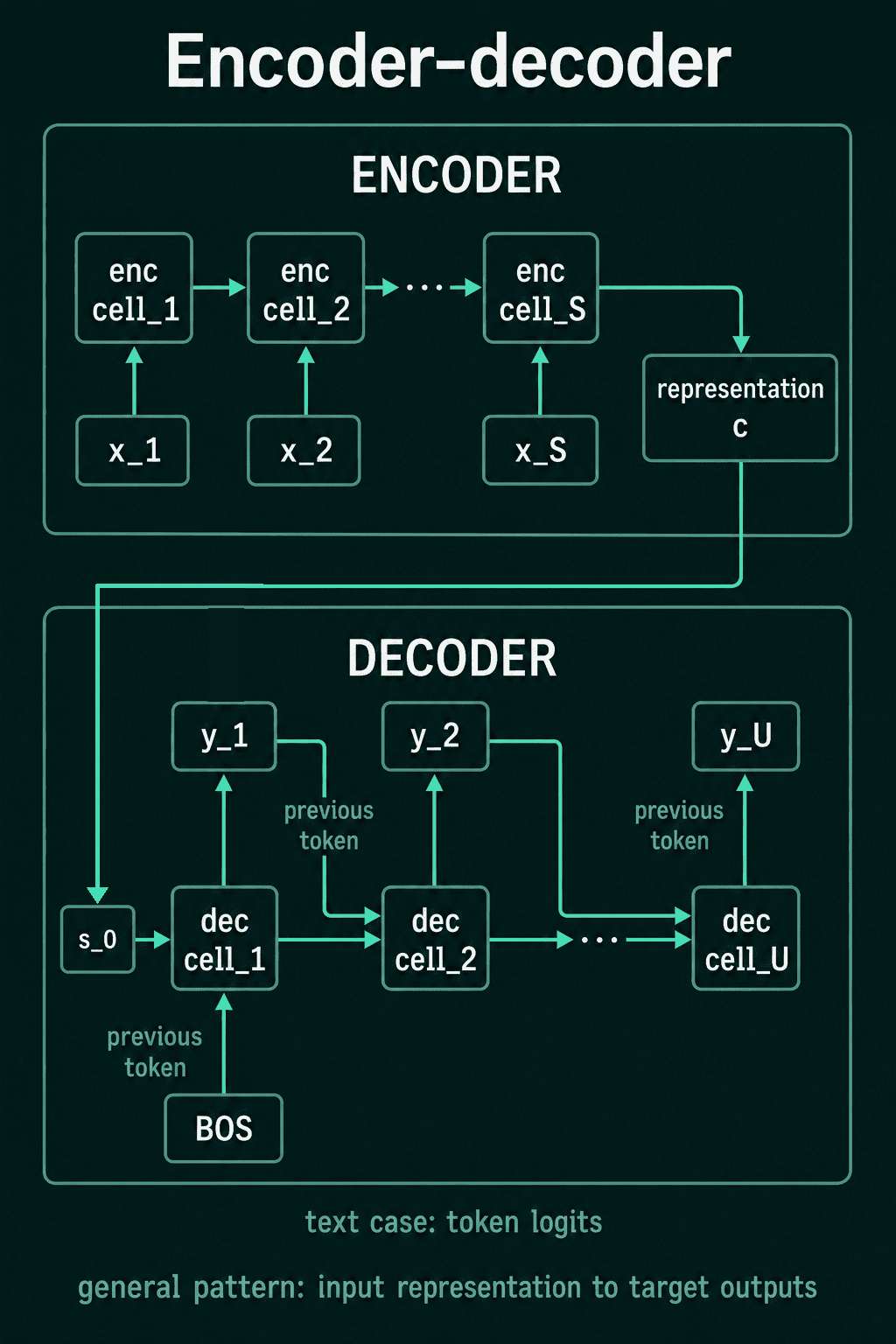
In the basic RNN version, the encoder compresses the whole source sequence into one context vector $\mathbf{c}$, its final hidden state:

$$\mathbf{c} = \mathbf{h}^{\text{enc}}_S$$

The decoder uses that context as its starting state:

$$\mathbf{s}_0 = \mathbf{c}$$

Each target step then runs the decoder update and the vocabulary head. The probability of each target token is now conditioned on the whole source sequence $\mathbf{x}_{1:S}$, because the source reached the decoder through $\mathbf{s}_0$:

$$P(y_u \mid y_{<u}, \mathbf{x}_{1:S}) = \mathrm{softmax}(\mathbf{W}_{\text{out}}\mathbf{s}_u + \mathbf{b}_{\text{out}})$$

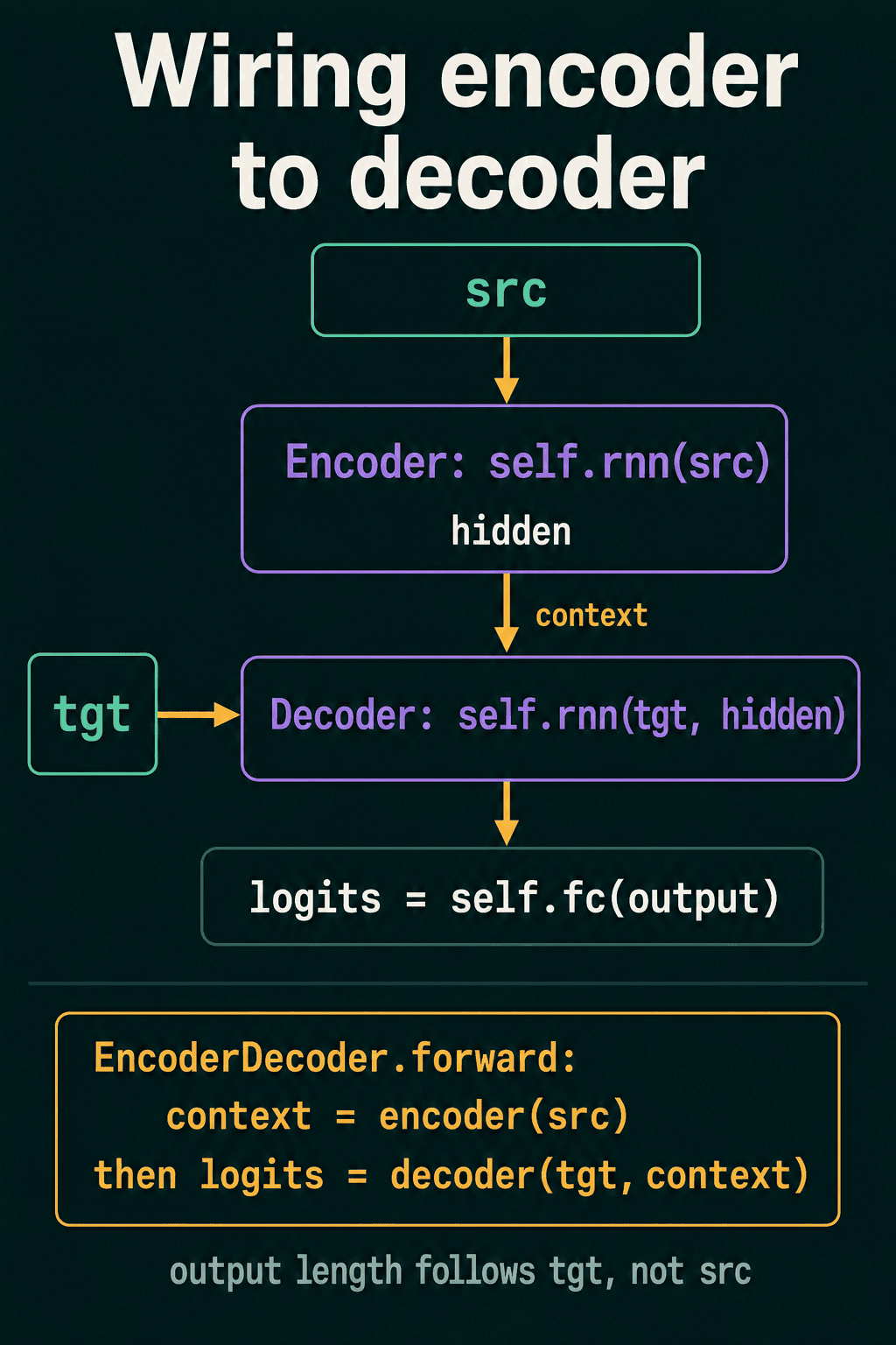
The encoder loop runs over the $S$ source positions and the decoder loop runs over the $U$ target positions. $S$ and $U$ do not have to match, which is what lets the model handle four English words in and two German words out.

The combined model wires the two parts together. Here the encoder returns hidden with its layer dimension still in place, because that is the shape nn.RNN expects as a starting state:

1class Encoder(nn.Module):
2    def __init__(self, input_size, hidden_size):
3        super().__init__()
4        self.rnn = nn.RNN(input_size, hidden_size, batch_first=True)
5 
6    def forward(self, src):
7        output, hidden = self.rnn(src)
8        return hidden
9 
10class Decoder(nn.Module):
11    def __init__(self, input_size, hidden_size, vocab_size):
12        super().__init__()
13        self.rnn = nn.RNN(input_size, hidden_size, batch_first=True)
14        self.fc = nn.Linear(hidden_size, vocab_size)
15 
16    def forward(self, tgt, hidden):
17        output, hidden = self.rnn(tgt, hidden)
18        logits = self.fc(output)
19        return logits, hidden
20 
21class EncoderDecoder(nn.Module):
22    def __init__(self, encoder, decoder):
23        super().__init__()
24        self.encoder = encoder
25        self.decoder = decoder
26 
27    def forward(self, src, tgt):
28        context = self.encoder(src)
29        logits, _ = self.decoder(tgt, context)
30        return logits
31 
32model = EncoderDecoder(
33    Encoder(input_size=64, hidden_size=128),
34    Decoder(input_size=64, hidden_size=128, vocab_size=1000),
35)
36src = torch.rand(4, 10, 64)  # 4 source sentences, 10 tokens each
37tgt = torch.rand(4, 8, 64)   # 4 target inputs, 8 tokens each
38print(model.encoder(src).shape)
39print(model(src, tgt).shape)

1torch.Size([1, 4, 128])
2torch.Size([4, 8, 1000])

The source has 10 tokens and the target has 8, and the logits come out with 8 steps. The output length follows tgt, because the decoder produces one logits vector per target-side input.

The bottleneck of one context vector

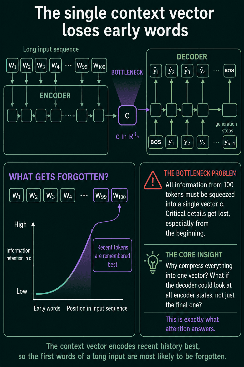
A recurrent network's hidden state has a fixed size no matter how long the input is. LSTMs and GRUs have gates that help carry information through time, but their state is still a fixed number of values. In a basic encoder-decoder, the same limit shows up between the two networks. Everything the decoder needs about the source has to pass through the one vector $\mathbf{c}$, including what the tokens say, their order and how they relate to each other.

For short inputs this can work well. For long inputs, the encoder may lose details from the start of the sequence before the decoder ever begins, because the last tokens it read tend to be represented best in its final state.

A fix is to let the decoder look back at all the encoder states and pick the ones it needs for each output step, instead of receiving only the final one. That is what attention does, and it is a step from this basic model toward the transformer.

Common mistakes

• Passing the summary as the decoder's starting state. hn[-1] has shape (batch, hidden), and nn.RNN wants (layers, batch, hidden). Passing the 2-D summary with 3-D target inputs raises a RuntimeError.
• Assuming batch_first changes the state's shape. batch_first=True changes the layout of the input and output only. The hidden state is (layers, batch, hidden) either way.
• Expecting the output length to follow the source. The logits have one row per target-side input, so their length follows tgt.
• Leaving out the start token. The first decoder step needs a previous token too, so the target-side inputs begin with a start token such as BOS.
• Expecting one context vector to hold a long input. The fixed size of $\mathbf{c}$ limits how much of a long source the decoder can use, which is the problem attention addresses.

Related concepts

The RNN post covers the recurrent update that both the encoder and the decoder use here. An encoder-decoder can use LSTM or GRU cells in place of the plain RNN. With LSTM cells, the encoder's final state is the pair (hn, cn) and the decoder starts from both. Attention removes the single-vector handoff by letting each decoder step read every encoder state. Choosing which token to feed back during generation is its own topic, with methods such as greedy decoding, sampling and beam search.

QuiddityML teaches encoders, decoders and the encoder-decoder model as three concepts in the language models unit of its NLP track. The exercises include ordering the lines of RNNEncoder, following tensor shapes from src and tgt to the logits and writing the full encoder-decoder from scratch (QuiddityML).