By Sagi Shaier · 4 November 2026 · 10 min read

LSTM explained

One LSTM step worked by hand with real numbers, why its cell state helps gradients reach tokens further back in a sequence, and how to code it from scratch and with nn.LSTM in PyTorch.

A Long Short-Term Memory network (LSTM) is a recurrent neural network that passes two vectors from each step to the next, a hidden state and a cell state. Small learned switches called gates decide how much of the old memory to keep and how much new information to write. LSTMs were built to keep information across more steps than a plain recurrent network, and they were a common model for text, speech and time series before transformers.

What problem does an LSTM solve?

A recurrent neural network (RNN) reads a sequence one step at a time. In text, each step is one token, which is a whole word or a piece of a word turned into a vector of numbers. The RNN keeps one vector called the hidden state, written $\mathbf{h}_t$ at step $t$, and rewrites it at every step from the new input $\mathbf{x}_t$ and the previous hidden state.

The rewrite uses two learned weight matrices. $\mathbf{W}_h$ multiplies the previous hidden state and $\mathbf{W}_x$ multiplies the input. A learned bias vector $\mathbf{b}$ is added, and $\tanh$ squashes each entry of the result into the range from $-1$ to $1$:

$$\mathbf{h}_t = \tanh(\mathbf{W}_h \mathbf{h}_{t-1} + \mathbf{W}_x \mathbf{x}_t + \mathbf{b})$$

The same $\mathbf{W}_h$ and the same $\tanh$ are applied at every step. Information from step 1 has to survive being rewritten at step 2, then at step 3, and so on.

Training makes this harder. To learn that token 1 changed a prediction at step 20, the gradient has to travel back through 19 of those rewrites. Each one multiplies it by $\mathbf{W}_h$ and by the slope of $\tanh$. If those factors cut the gradient in half at each step, 20 steps leave $0.5^{20} \approx 0.00000095$ of it. This is the vanishing gradient problem. The model gets almost no training signal from distant tokens, so it mostly learns short-range patterns.

An LSTM keeps the step-by-step reading and adds a separate memory path that gradients can cross with much less shrinking.

The hidden state and the cell state

A plain RNN carries one state from step to step. An LSTM carries two:

The hidden state $\mathbf{h}_t$ is the vector the LSTM outputs at step $t$. It goes to the next step and to any prediction layer, such as a classifier.
The cell state $\mathbf{c}_t$ is a separate memory vector. It also goes to the next step, and the LSTM changes it only by keeping part of the old memory and adding part of some new content.

Both vectors have the same length, called the hidden size, which you pick when you build the model.

The three gates

A gate is a vector of numbers between 0 and 1 that multiplies another vector entry by entry. An entry of 1 lets that number through unchanged, 0 blocks it and 0.5 halves it. For example, multiplying $[0.8, -0.5]$ entry by entry with the gate $[1, 0]$ gives $[0.8, 0]$. This entry-by-entry product is written $\odot$.

Gates get their range from the sigmoid function $\sigma$, which maps any number to a value between 0 and 1. For example, $\sigma(-2) \approx 0.12$, $\sigma(0) = 0.5$ and $\sigma(2) \approx 0.88$. Each gate is computed again at every step from the current input and the previous hidden state, so the LSTM can keep a memory entry at one step and overwrite it at the next.

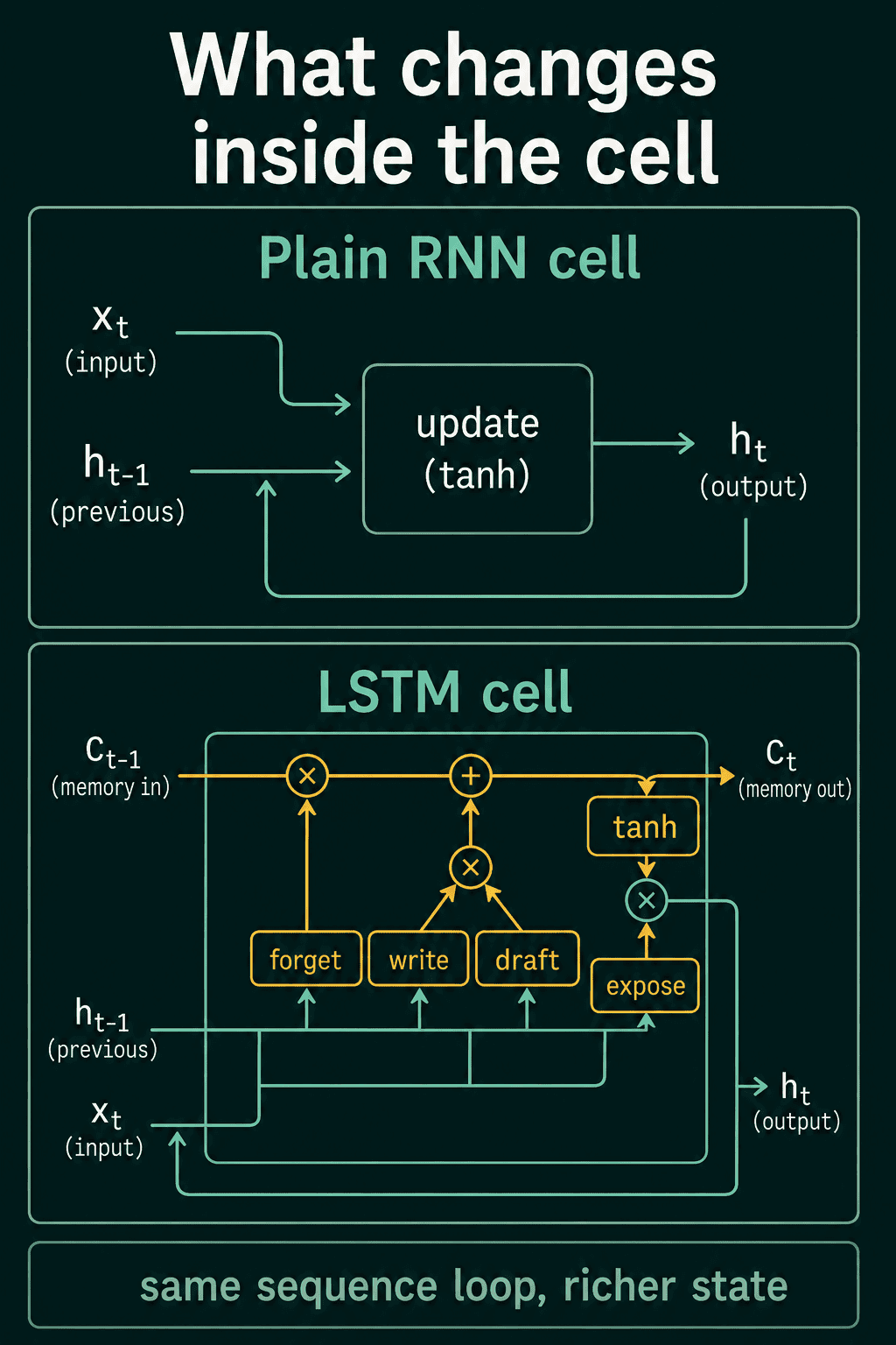
An LSTM has three gates and one extra vector:

The forget gate $\mathbf{f}_t$ sets what fraction of each entry of the old cell state survives.
The input gate $\mathbf{i}_t$ sets how much new content gets written into the cell state.
The candidate $\tilde{\mathbf{c}}_t$ is that new content. It is not a gate. It comes from $\tanh$, so its entries lie between $-1$ and $1$ and can be negative.
The output gate $\mathbf{o}_t$ sets how much of the updated cell state shows up in the hidden state.

The diagram below names each part by its job. "Forget" is the forget gate, "write" is the input gate, "draft" is the candidate and "expose" is the output gate.

A plain RNN cell with one tanh update box next to an LSTM cell, where the memory line runs from c_(t-1) to c_t across the top, forget scales the old memory, write times draft is added, and expose picks what leaves as h_t.

The LSTM equations

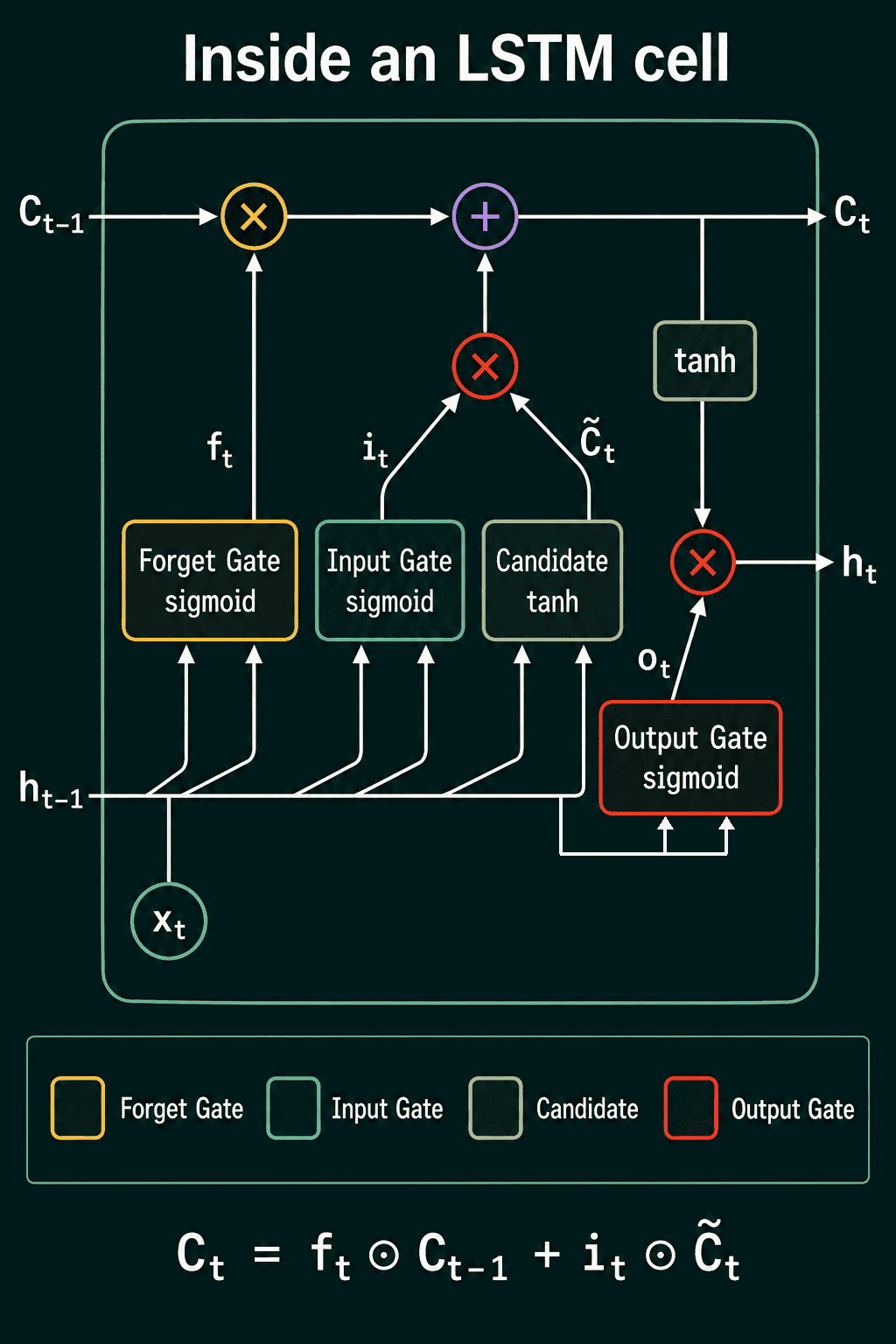
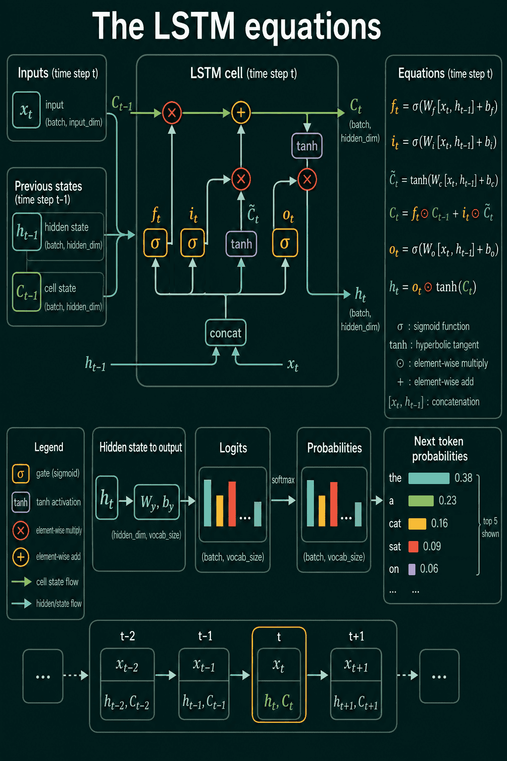
At step $t$ the LSTM receives the input $\mathbf{x}_t$ and the two previous states $\mathbf{h}_{t-1}$ and $\mathbf{c}_{t-1}$. The notation $[\mathbf{x}_t, \mathbf{h}_{t-1}]$ means the two vectors joined end to end into one longer vector. For example, $\mathbf{x}_t = [1, 2]$ and $\mathbf{h}_{t-1} = [0.5, -1]$ join into $[1, 2, 0.5, -1]$.

Each gate has its own weight matrix $\mathbf{W}$ and bias vector $\mathbf{b}$. Every $\mathbf{W}$ has shape (hidden_size, input_size + hidden_size), so it maps the joined vector back down to the hidden size. The forget gate, the input gate and the candidate all read the same joined vector:

$$\mathbf{f}_t = \sigma(\mathbf{W}_f [\mathbf{x}_t, \mathbf{h}_{t-1}] + \mathbf{b}_f)$$

$$\mathbf{i}_t = \sigma(\mathbf{W}_i [\mathbf{x}_t, \mathbf{h}_{t-1}] + \mathbf{b}_i)$$

$$\tilde{\mathbf{c}}_t = \tanh(\mathbf{W}_c [\mathbf{x}_t, \mathbf{h}_{t-1}] + \mathbf{b}_c)$$

The new cell state keeps the surviving part of the old memory and adds the admitted part of the candidate:

$$\mathbf{c}_t = \mathbf{f}_t \odot \mathbf{c}_{t-1} + \mathbf{i}_t \odot \tilde{\mathbf{c}}_t$$

The output gate reads the same joined vector. The hidden state is the output gate applied to the $\tanh$ of the new cell state:

$$\mathbf{o}_t = \sigma(\mathbf{W}_o [\mathbf{x}_t, \mathbf{h}_{t-1}] + \mathbf{b}_o)$$

$$\mathbf{h}_t = \mathbf{o}_t \odot \tanh(\mathbf{c}_t)$$

Each step makes three choices in order. It keeps part of the old memory, writes new memory, then shows part of that memory as $\mathbf{h}_t$.

Inside an LSTM cell: c_(t-1) runs along the top through a multiply with the forget gate f_t and an add with the input gate i_t times the candidate, h_(t-1) and x_t feed all four gate boxes, and the output gate o_t times tanh(c_t) gives h_t.

In a language model, $\mathbf{h}_t$ then goes through one more linear layer with weights $\mathbf{W}_y$ and bias $\mathbf{b}_y$. That layer gives one score per token in the vocabulary, and these scores are called logits. The softmax function turns the logits into probabilities for the next token.

The LSTM equations next to the cell diagram, with h_t passed through W_y and b_y to logits, softmax turning them into probabilities, a top-5 next-token list led by "the" at 0.38, and the same cell repeated over steps t-2 to t+1.

One step by hand

Take a hidden size of 2, and suppose the gates and the candidate at one step come out as follows. The old cell state is $\mathbf{c}_{t-1} = [0.8, -0.5]$. The forget gate is $\mathbf{f}_t = [0.9, 0.1]$, the input gate is $\mathbf{i}_t = [0.2, 0.7]$ and the candidate is $\tilde{\mathbf{c}}_t = [0.5, 0.6]$.

The kept part of the old memory is $\mathbf{f}_t \odot \mathbf{c}_{t-1} = [0.72, -0.05]$. The written part is $\mathbf{i}_t \odot \tilde{\mathbf{c}}_t = [0.10, 0.42]$. Adding them gives the new cell state:

$$\mathbf{c}_t = [0.82, 0.37]$$

The two entries behave differently. In the first, the forget gate of 0.9 kept most of the old 0.8 and the input gate of 0.2 added a little. In the second, the forget gate of 0.1 dropped most of the old $-0.5$ and the input gate of 0.7 wrote most of the candidate's 0.6, so that memory entry went from negative to positive.

With an output gate of $\mathbf{o}_t = [0.5, 0.9]$, the hidden state is $\mathbf{o}_t \odot \tanh(\mathbf{c}_t)$. Since $\tanh(\mathbf{c}_t) \approx [0.675, 0.354]$, the result is about $[0.338, 0.319]$. The same step in PyTorch:

1import torch
2 
3c_prev = torch.tensor([0.8, -0.5])
4f = torch.tensor([0.9, 0.1])        # forget gate
5i = torch.tensor([0.2, 0.7])        # input gate
6c_tilde = torch.tensor([0.5, 0.6])  # candidate
7o = torch.tensor([0.5, 0.9])        # output gate
8 
9c = f * c_prev + i * c_tilde
10h = o * torch.tanh(c)
11print(c)
12print(h)

1tensor([0.8200, 0.3700])
2tensor([0.3375, 0.3186])

Why the cell state helps with vanishing gradients

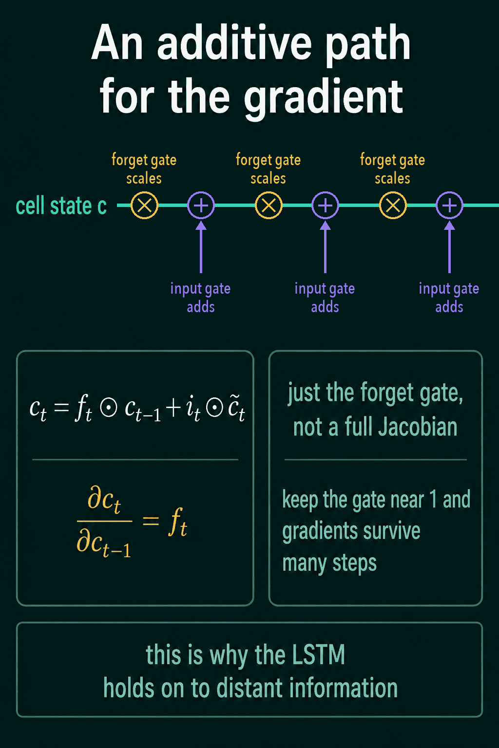
The cell state update adds its two parts. The old memory reaches $\mathbf{c}_t$ through one multiplication by the forget gate, with no weight matrix and no $\tanh$ on that path. So along this direct path the derivative of $\mathbf{c}_t$ with respect to $\mathbf{c}_{t-1}$, entry by entry, is the forget gate itself:

$$\frac{\partial \mathbf{c}_t}{\partial \mathbf{c}_{t-1}} = \mathbf{f}_t$$

In a plain RNN, each backward step multiplies the gradient by a Jacobian, the matrix of derivatives of every entry of $\mathbf{h}_t$ with respect to every entry of $\mathbf{h}_{t-1}$. That matrix contains $\mathbf{W}_h$ and the slope of $\tanh$ at every step. On the LSTM's cell-state path, each backward step multiplies by the forget gate only.

When a forget gate entry stays near 1, the gradient on that entry shrinks very little. A forget gate of 0.95 held for 20 steps keeps $0.95^{20} \approx 0.36$ of the gradient, and 0.99 keeps about 0.82. Compare that with the $0.00000095$ left after 20 halvings. The model still has to learn to hold the forget gate open for information worth keeping, so long-range learning gets easier without becoming automatic. Skip connections in deep networks rely on the same idea, an added path that lets gradients go around a transformation that would shrink them.

The cell state line passing through three steps, each with a forget-gate multiply and an input-gate add, above the update c_t = f_t ⊙ c_(t-1) + i_t ⊙ c̃_t and its derivative ∂c_t/∂c_(t-1) = f_t.

Coding an LSTM cell from scratch

The equations turn into one step of code. LSTMCell takes the current input, the previous hidden state and the previous cell state, then returns the updated pair. Each nn.Linear(input_size + hidden_size, hidden_size) holds one gate's $\mathbf{W}$ and $\mathbf{b}$.

1import torch
2import torch.nn as nn
3 
4class LSTMCell(nn.Module):
5    def __init__(self, input_size, hidden_size):
6        super().__init__()
7        self.W_f = nn.Linear(input_size + hidden_size, hidden_size)
8        self.W_i = nn.Linear(input_size + hidden_size, hidden_size)
9        self.W_c = nn.Linear(input_size + hidden_size, hidden_size)
10        self.W_o = nn.Linear(input_size + hidden_size, hidden_size)
11 
12    def forward(self, x, h, c):
13        combined = torch.cat([x, h], dim=1)
14        f = torch.sigmoid(self.W_f(combined))
15        i = torch.sigmoid(self.W_i(combined))
16        c_tilde = torch.tanh(self.W_c(combined))
17        o = torch.sigmoid(self.W_o(combined))
18        c = f * c + i * c_tilde
19        h = o * torch.tanh(c)
20        return h, c

torch.cat([x, h], dim=1) is the joined vector $[\mathbf{x}_t, \mathbf{h}_{t-1}]$ for every sequence in the batch. The previous cell state skips that join and goes straight into the update line.

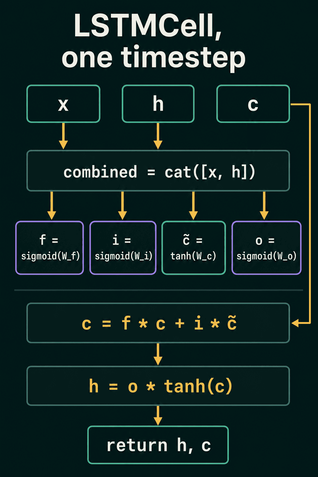
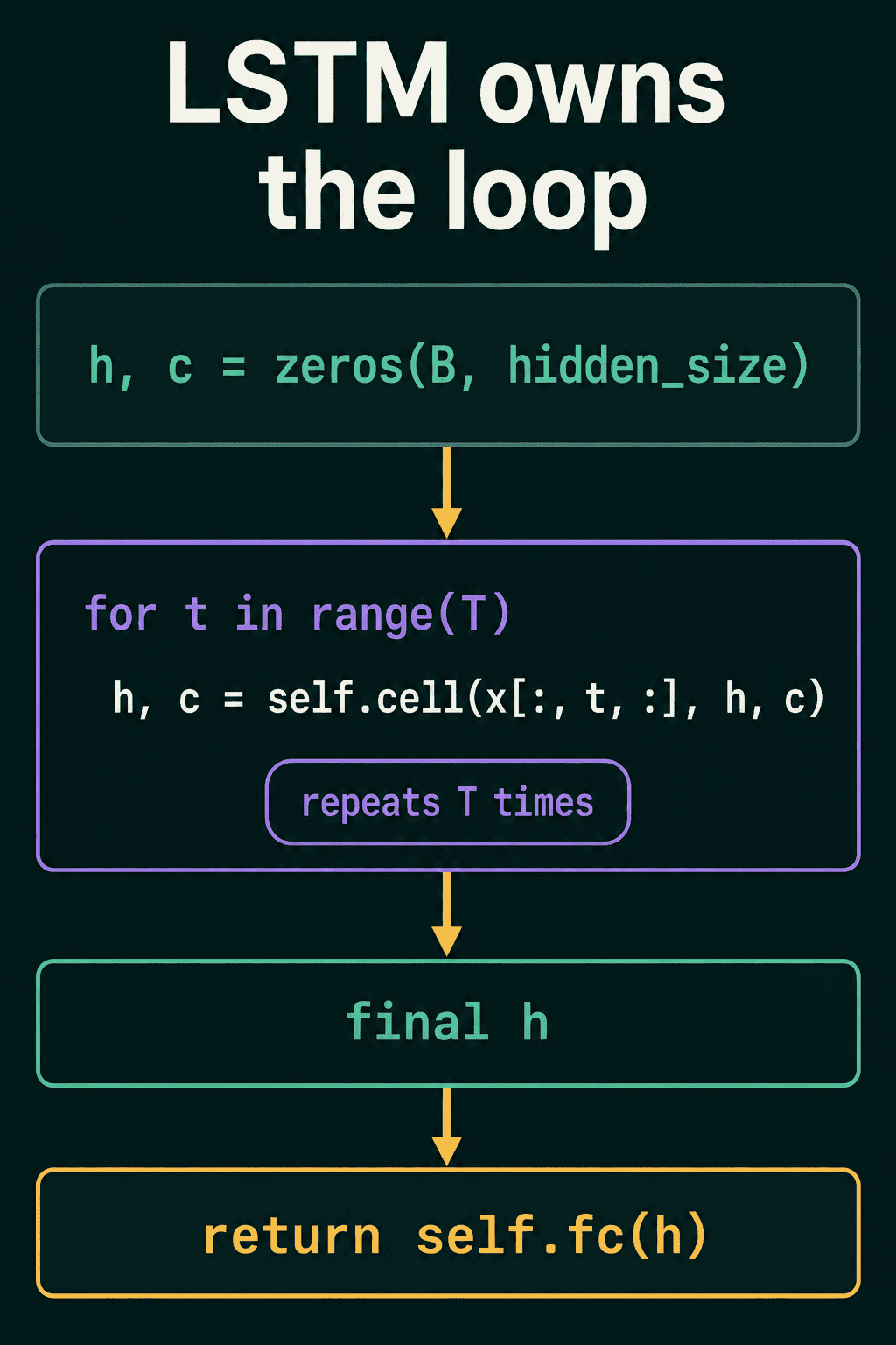
LSTMCell for one timestep: x and h joined by cat into combined, four gate boxes computed from it, and c passed around the side into c = f * c + i * c̃, followed by h = o * tanh(c) and return h, c.

The cell handles one step. An outer model owns the loop over steps, the starting states and a classifier head:

1class LSTM(nn.Module):
2    def __init__(self, input_size, hidden_size, num_classes):
3        super().__init__()
4        self.hidden_size = hidden_size
5        self.cell = LSTMCell(input_size, hidden_size)
6        self.fc = nn.Linear(hidden_size, num_classes)
7 
8    def forward(self, x):
9        B, T, _ = x.shape
10        h = torch.zeros(B, self.hidden_size, device=x.device)
11        c = torch.zeros(B, self.hidden_size, device=x.device)
12        for t in range(T):
13            h, c = self.cell(x[:, t, :], h, c)
14        return self.fc(h)
15 
16torch.manual_seed(0)
17model = LSTM(input_size=8, hidden_size=16, num_classes=3)
18x = torch.randn(4, 10, 8)  # 4 sequences, 10 steps, 8 numbers per step
19print(model(x).shape)

1torch.Size([4, 3])

Both states start at zeros, and the loop calls the cell once per step. The classifier reads only the final hidden state, which is called a many-to-one setup because many inputs produce one output.

The outer LSTM model: h and c start as zeros, a loop over t calls self.cell T times, and the final h goes into self.fc.

nn.LSTM in PyTorch

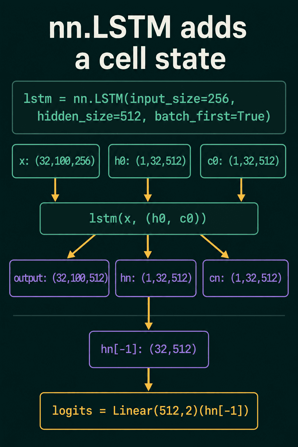
PyTorch has the whole recurrent layer built in as nn.LSTM. It runs the same gated update inside and returns the hidden state for every step. The interface change from nn.RNN is the state. nn.RNN returns output, hn, while nn.LSTM returns output, (hn, cn) because it carries both states.

1import torch
2import torch.nn as nn
3 
4lstm = nn.LSTM(input_size=256, hidden_size=512, batch_first=True)
5 
6x = torch.randn(32, 100, 256)  # 32 sequences, 100 steps, 256 numbers per step
7h0 = torch.zeros(1, 32, 512)
8c0 = torch.zeros(1, 32, 512)
9 
10output, (hn, cn) = lstm(x, (h0, c0))
11logits = nn.Linear(512, 2)(hn[-1])
12 
13print(output.shape)
14print(hn.shape, cn.shape)
15print(logits.shape)

1torch.Size([32, 100, 512])
2torch.Size([1, 32, 512]) torch.Size([1, 32, 512])
3torch.Size([32, 2])

batch_first=True means the input is laid out as (batch, steps, features). output holds one hidden state per step, which a tagging model would read. The first dimension of hn and cn counts layers, so hn[-1] is the last layer's final hidden state, ready for a classifier. cn is the final cell state, which you need when another recurrent module has to continue from the same memory. If you leave out (h0, c0), PyTorch starts both states at zeros.

nn.LSTM with input_size 256 and hidden_size 512: x of shape (32, 100, 256), h0 and c0 of shape (1, 32, 512) go in, output of shape (32, 100, 512), hn and cn of shape (1, 32, 512) come out, and hn[-1] of shape (32, 512) feeds Linear(512, 2).

When to use an LSTM

In classic recurrent NLP the LSTM was the more common default. If you are using a recurrent model and have no tight limit on size or speed, an LSTM is a reasonable place to start. A GRU is a smaller recurrent cell with two gates and one state, and the LSTM vs GRU post compares the two.

In modern NLP, LSTMs and GRUs are much less central than transformers. They are still used for small models, streaming input, devices with little memory and time-series data. The reason is cost. Attention compares every pair of positions in a sequence, while a recurrent model processes the sequence with a fixed-size state.

Common mistakes

Unpacking nn.LSTM like nn.RNN. output, hn = lstm(x) runs without an error, but hn is then the tuple (hn, cn) and the next line that uses it as a tensor fails.
Passing h0 without c0. nn.LSTM expects the starting state as a tuple (h0, c0), and passing h0 alone raises an error.
Reading cn as the output. Predictions read hn[-1] or output. The cell state is the LSTM's internal memory.
Mixing up the input layout. With batch_first=True the input is (batch, steps, features), and without it the input is (steps, batch, features).
Expecting unlimited memory. The cell state has a fixed size, and the gates still have to learn what to keep. Long inputs can lose early details.

The RNN post covers the plain recurrent update, backpropagation through time and why its gradients vanish. nn.LSTM takes the same bidirectional and num_layers arguments as nn.RNN, so a bidirectional or stacked LSTM needs one extra argument. The GRU drops the separate cell state and uses two gates. The encoder-decoder post shows how two recurrent networks join up for tasks such as translation.

QuiddityML teaches the LSTM in the language models unit of its NLP track. Its exercises include matching each gate equation to its line of code, following the gradient along the cell-state path and writing LSTMCell from scratch (QuiddityML).