By Sagi Shaier · 9 October 2026 · 5 min read

Least squares explained: linear regression as a projection, and the normal equation

How least squares becomes a projection onto a column space, how the normal equations come out of one orthogonality condition, what the Gram matrix is and when it fails, and how to fit a line in PyTorch.

Least squares finds the input $\mathbf{x}$ that makes $A\mathbf{x}$ as close as possible to a target $\mathbf{b}$ when no input hits it exactly. Linear regression is least squares: with more data points than unknowns, no line passes through every point, and least squares picks the line whose squared errors add up to the smallest total.

Why there is usually no exact solution

Fitting a line $y = c_0 + c_1 x$ to five points means finding two numbers, $c_0$ and $c_1$, that satisfy five equations, one per point. Stack the equations as $A\mathbf{x} = \mathbf{b}$: each row of $A$ is $(1, x_i)$, $\mathbf{x} = (c_0, c_1)$ holds the unknowns, and $\mathbf{b}$ holds the five $y$ values.

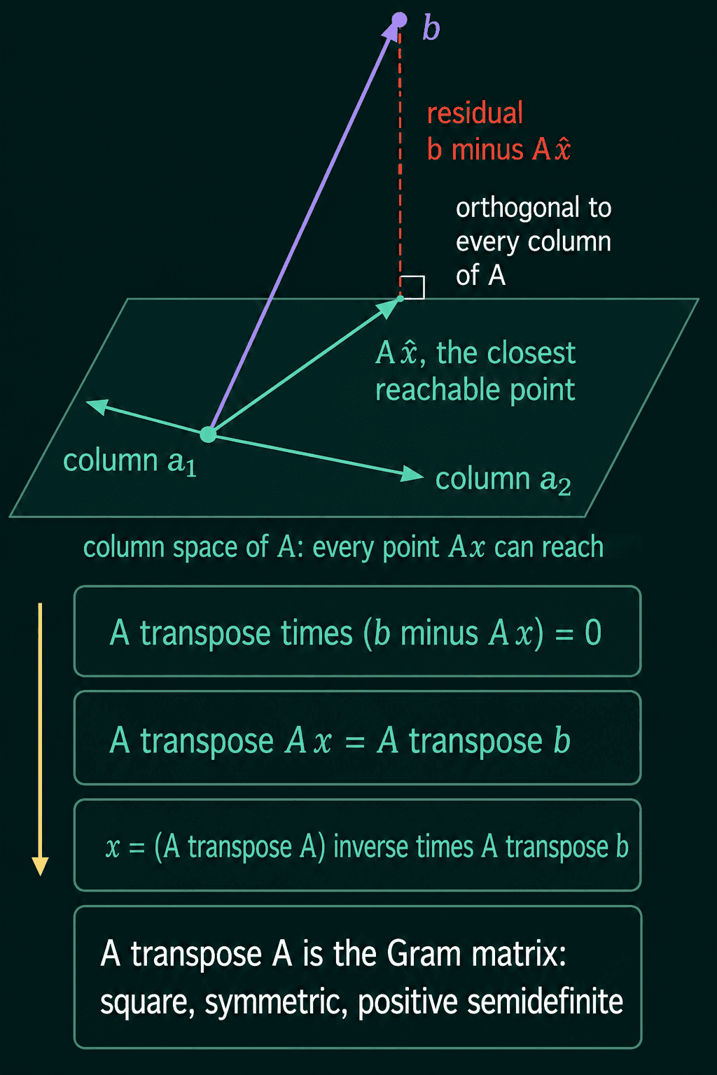
The column space of $A$ is the set of every vector $A\mathbf{x}$ can produce, which here is every set of five values that lie exactly on some line. Real data rarely lies exactly on a line, so $\mathbf{b}$ is usually outside the column space and $A\mathbf{x} = \mathbf{b}$ has no solution.

The next best thing is the point in the column space closest to $\mathbf{b}$. Finding the closest point in a set to a given vector is a projection.

The residual has to be orthogonal

Call the best input $\hat{\mathbf{x}}$, so $A\hat{\mathbf{x}}$ is the closest reachable point. The residual $\mathbf{b} - A\hat{\mathbf{x}}$ is the gap between the target and that point, one error per data point.

At the closest point, the residual is orthogonal (at a right angle) to every direction you can move inside the column space, which means its dot product with every column of $A$ is zero. If it had a part along some column, moving along that column would shrink the gap. One matrix equation checks every column at once, where $A^\top$ is the transpose of $A$:

$$A^\top(\mathbf{b} - A\hat{\mathbf{x}}) = 0$$

The target b above a plane spanned by the columns a1 and a2 of A, with A x-hat the closest point in the plane and the dashed residual from A x-hat up to b at a right angle to every column, above the steps from A transpose times the residual equals 0 to the normal equations

The normal equations

Multiply out the brackets and move the $\hat{\mathbf{x}}$ term to the other side:

$$A^\top A\,\hat{\mathbf{x}} = A^\top \mathbf{b}$$

These are the normal equations. When $A^\top A$ has an inverse:

$$\hat{\mathbf{x}} = (A^\top A)^{-1} A^\top \mathbf{b}$$

and the closest point itself, the projection of $\mathbf{b}$ onto the column space, is:

$$A\hat{\mathbf{x}} = A(A^\top A)^{-1} A^\top \mathbf{b}$$

This $\hat{\mathbf{x}}$ is what linear regression solves for: the line, plane, or higher-dimensional plane closest to data that does not sit on any of them.

The Gram matrix

$A^\top A$ comes up often enough to have a name, the Gram matrix of $A$. Its entry in row $i$ and column $j$ is the dot product of column $i$ and column $j$ of $A$. It is always square, and always symmetric, since $(A^\top A)^\top = A^\top A$.

It is also positive semidefinite, meaning $\mathbf{z}^\top (A^\top A)\,\mathbf{z} \geq 0$ for every vector $\mathbf{z}$. That expression rearranges into a squared length:

$$\mathbf{z}^\top (A^\top A)\,\mathbf{z} = (A\mathbf{z})^\top (A\mathbf{z}) = \|A\mathbf{z}\|^2$$

and a squared length is never negative. It equals 0 only when $A\mathbf{z} = 0$.

When the columns of $A$ are linearly independent (none of them is a combination of the others, also called full column rank), $A\mathbf{z} = 0$ only for $\mathbf{z} = 0$. Then $\mathbf{z}^\top (A^\top A)\,\mathbf{z}$ is strictly positive for every nonzero $\mathbf{z}$, and $A^\top A$ has an inverse. If one column is a combination of the others, for example one feature that is twice another, the Gram matrix is singular and the formula above breaks.

Fitting a line in PyTorch

Five points $(0, 1), (1, 3), (2, 4), (3, 4), (4, 7)$ do not sit on one line:

1import torch
2 
3# five points that do not sit on one line
4x = torch.tensor([0.0, 1.0, 2.0, 3.0, 4.0])
5b = torch.tensor([1.0, 3.0, 4.0, 4.0, 7.0])
6A = torch.stack([torch.ones_like(x), x], dim=1)   # columns: intercept, slope
7 
8G = A.T @ A                                       # Gram matrix
9print(G)
10coef = torch.linalg.solve(G, A.T @ b)             # normal equations
11print(coef)
12print(torch.linalg.lstsq(A, b.unsqueeze(1)).solution.squeeze())
13 
14r = b - A @ coef
15print((A.T @ r).round(decimals=4))                # residual orthogonal to every column

1tensor([[ 5., 10.],
2        [10., 30.]])
3tensor([1.2000, 1.3000])
4tensor([1.2000, 1.3000])
5tensor([0., 0.])

The best line is $y = 1.2 + 1.3x$. torch.linalg.solve(G, A.T @ b) solves the normal equations without forming the inverse, and torch.linalg.lstsq(A, b) solves the least squares problem directly from $A$ and $\mathbf{b}$. The last line confirms the orthogonality condition: the residual has a dot product of 0 with both columns.

When a column is a combination of the others, the Gram matrix has a zero eigenvalue (a direction it sends to zero):

1import torch
2 
3x = torch.tensor([0.0, 1.0, 2.0, 3.0, 4.0])
4A = torch.stack([torch.ones_like(x), x, 2 * x], dim=1)   # third column = 2 * second
5G = A.T @ A
6print(torch.linalg.matrix_rank(A))
7print(torch.linalg.eigvalsh(G).round(decimals=4))

1tensor(2)
2tensor([ -0.0000,   1.6300, 153.3700])

Three columns with rank 2 mean one column adds nothing new, and the zero eigenvalue means $A^\top A$ has no inverse. If a fit returns huge or unstable coefficients, check the rank of $A$ first, since near-duplicate features cause the same problem in a milder form.

When to use the normal equations, and when not to

The normal equations give the exact least squares answer in one step, which suits small and medium problems. For numerical work, torch.linalg.lstsq is usually the better call: forming $A^\top A$ squares how sensitive the problem is to rounding errors, while lstsq works from $A$ directly. Computing torch.linalg.inv(A.T @ A) explicitly is the least stable option of the three.

Common mistakes:

Forgetting the column of ones. Without it the fitted line is forced through the origin.
Inverting a singular Gram matrix. Duplicate or proportional features make $A^\top A$ singular, and the inverse either fails or returns huge numbers.
Mixing up $A^\top A$ and $A A^\top$. The normal equations use $A^\top A$, which has one row and column per unknown.
Expecting the residual to be zero. It is zero only when the points already sit on a line. Least squares makes it as small as possible, and orthogonal to the columns.

Projection onto a single direction and orthogonality are covered in orthogonality explained, and least squares is the same idea applied to a whole column space. Rank and column space are in rank, column space and null space explained. Multicollinearity is the near-singular case of the Gram matrix, covered in multicollinearity explained.

QuiddityML teaches least squares as its own concept in the linear algebra part of the Math track, and the exercises include turning the normal equations into code, tracing a fit on a small matrix by hand, and writing least_squares from scratch.