By Sagi Shaier · 21 October 2026 · 7 min read

Mutual information explained

How to compute mutual information from a joint probability table by hand and in PyTorch, how it connects to entropy and KL divergence, and where it is used in feature selection and decision trees.

Mutual information measures how much knowing the value of one variable reduces your uncertainty about another. It is 0 when the two variables are unrelated, and it picks up relationships of any shape, including ones that a correlation coefficient scores as 0.

What problem does mutual information solve?

Correlation measures how well a straight line describes the relationship between two variables. Take $X$ equal to $-1$, $0$ or $1$ with probability 1/3 each, and set $Y = X^2$. Knowing $X$ tells you $Y$ exactly, yet the correlation between them is exactly 0, because $Y$ goes up on both sides of $X = 0$ and the two halves cancel.

Mutual information measures how much less uncertain you are about $Y$ after you learn $X$. For $Y = X^2$, once $X$ is known there is no uncertainty left about $Y$, so the mutual information is as large as it can be for this $Y$, about 0.637 nats. The PyTorch section below computes it next to the correlation.

Entropy, the starting point

Uncertainty here is measured with entropy. For a variable $Y$ whose values have probabilities $p(y)$, the entropy is

$$H(Y) = -\sum_y p(y) \log p(y)$$

It is 0 when one value is certain and largest when all values are equally likely. With the natural log the unit is the nat. A fair coin has entropy $\ln 2 \approx 0.693$ nats.

Joint, marginal and conditional distributions

Mutual information needs three ways of describing two variables. Take $X$ and $Y$ that are each 0 or 1:

The joint distribution $p(x, y)$ gives the probability of each pair of values together. Here the pairs $(0, 0)$ and $(1, 1)$ each have probability 0.4 and the pairs $(0, 1)$ and $(1, 0)$ each have 0.1, so $X$ and $Y$ agree 80% of the time.
A marginal like $p(x)$ is the joint summed over every value of the other variable. $p(X{=}0) = 0.4 + 0.1 = 0.5$, and every marginal in this table comes out at 0.5.
A conditional like $p(y \mid x)$ is the distribution of $Y$ once $X$ is fixed. Given $X = 0$, the row $[0.4, 0.1]$ divided by its total 0.5 gives $p(y \mid X{=}0) = [0.8, 0.2]$.

Mutual information as a drop in entropy

Before learning anything, $Y$ is a fair coin, so $H(Y) = \ln 2 \approx 0.693$ nats. After learning $X$, the uncertainty left in $Y$ is the conditional entropy $H(Y \mid X)$: the entropy of each conditional distribution, averaged over the values of $X$ with weights $p(x)$:

$$H(Y \mid X) = \sum_x p(x)\, H(Y \mid X{=}x)$$

Here both conditionals are $[0.8, 0.2]$ or $[0.2, 0.8]$, and each has entropy

$$-(0.8 \ln 0.8 + 0.2 \ln 0.2) \approx 0.500 \text{ nats}$$

so their average is also 0.500 nats. Mutual information is the uncertainty that went away:

$$I(X; Y) = H(Y) - H(Y \mid X) \approx 0.693 - 0.500 = 0.193 \text{ nats}$$

Knowing $X$ removes about 28% of the uncertainty in $Y$. Independent variables give $I = 0$. If $Y$ is fully determined by $X$, the leftover uncertainty is 0 and $I = H(Y)$.

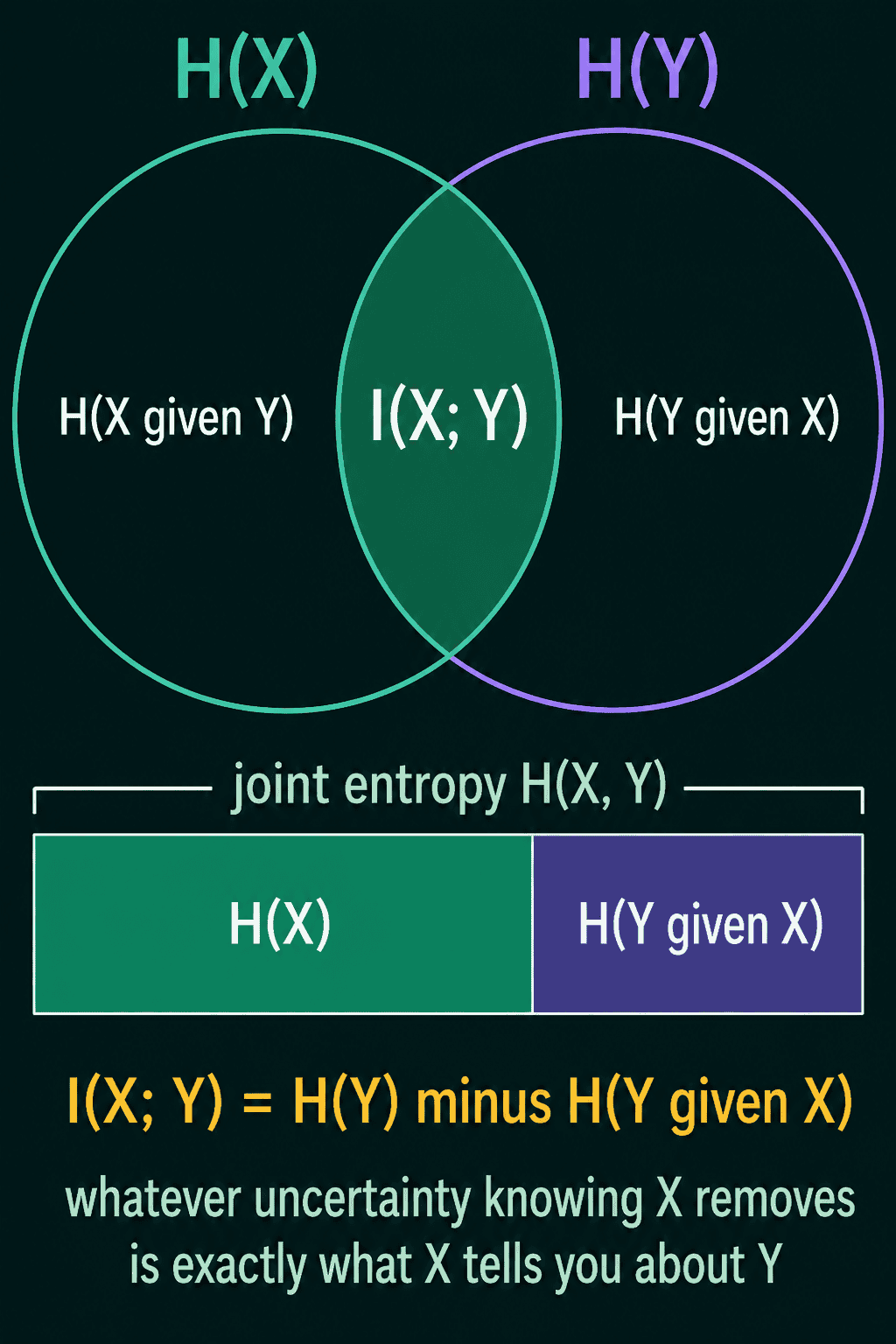
The same pieces add up for the pair as a whole. The joint entropy $H(X, Y)$ is the entropy formula applied directly to the four cells of the joint table, and it splits as

$$H(X, Y) = H(X) + H(Y \mid X)$$

The total uncertainty in the pair is the uncertainty in $X$, plus whatever is still left in $Y$ once $X$ is known. For the table above, $-(2 \cdot 0.4 \ln 0.4 + 2 \cdot 0.1 \ln 0.1) \approx 1.194$ nats, which matches $0.693 + 0.500$. The diagram below shows the overlap of the two entropies as $I(X; Y)$, where $H(X \mid Y)$ is the uncertainty left in $X$ once $Y$ is known:

Two overlapping circles labeled H(X) and H(Y), with the overlap labeled I(X; Y) and the rest labeled H(X given Y) and H(Y given X), above a bar showing the joint entropy H(X, Y) split into H(X) and H(Y given X).

Mutual information as a KL divergence

KL divergence measures how far one distribution $p$ is from another distribution $q$ over the same values, as $\sum p \log (p / q)$, and it is 0 only when the two are identical.

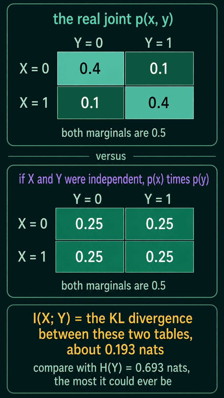
If $X$ and $Y$ were independent, their joint would be the product of the marginals, $p(x)p(y)$. Mutual information is the KL divergence between the real joint and that product:

$$I(X; Y) = \sum_{x, y} p(x, y) \log \frac{p(x, y)}{p(x)\, p(y)}$$

It measures how far the real table is from a table where the two variables have nothing to do with each other. In the example every marginal is 0.5, so the product table is 0.25 in every cell. The two 0.4 cells and the two 0.1 cells give

$$2\left[0.4 \ln \frac{0.4}{0.25} + 0.1 \ln \frac{0.1}{0.25}\right] \approx 0.193 \text{ nats}$$

the same 0.193 nats as before, out of a possible $H(Y) \approx 0.693$:

The real joint table with 0.4 on the diagonal and 0.1 off it, compared with the independent table of p(x) times p(y) with 0.25 in every cell, and their KL divergence of about 0.193 nats against H(Y) = 0.693 nats.

Three properties follow from this form:

It is symmetric: $I(X; Y) = I(Y; X)$, so the order of the two variables makes no difference. KL divergence on its own is not symmetric.
It is never negative. Learning another variable cannot leave you more uncertain on average.
It is 0 when $X$ and $Y$ are independent, because then the joint equals the product and every log is $\log 1 = 0$.

Mutual information in PyTorch

The KL form is the one to code, because it needs only the joint table. Summing the rows gives $p(x)$ and summing the columns gives $p(y)$. Multiplying them builds the independent table:

1import torch
2 
3def mutual_information(joint):
4    px = joint.sum(dim=1, keepdim=True)   # (n, 1), p(x): summed over Y
5    py = joint.sum(dim=0, keepdim=True)   # (1, m), p(y): summed over X
6    independent = px * py                 # (n, m), p(x)p(y) for every pair
7    mask = joint > 0                      # cells with p(x, y) = 0 add nothing
8    return (joint[mask] * torch.log(joint[mask] / independent[mask])).sum()
9 
10related = torch.tensor([[0.4, 0.1],
11                        [0.1, 0.4]])
12unrelated = torch.tensor([[0.25, 0.25],
13                          [0.25, 0.25]])
14copy = torch.tensor([[0.5, 0.0],
15                     [0.0, 0.5]])
16for name, joint in (("agree 80%", related), ("independent", unrelated), ("Y = X", copy)):
17    print(f"{name:12} {mutual_information(joint):.4f} nats")
18# agree 80%    0.1927 nats
19# independent  0.0000 nats
20# Y = X        0.6931 nats

When $Y$ is a copy of $X$, the mutual information reaches its cap $H(Y) = \ln 2$.

keepdim=True keeps the two marginals as a (n, 1) column and a (1, m) row, and multiplying a column by a row broadcasts into the full (n, m) table of every $p(x)p(y)$. Without it the sums come back as flat (n,) and (m,) tensors, and px * py multiplies them entry by entry into a vector of length 2 here, or raises a shape error when $n \neq m$.

Continuing from the code above, here is the $Y = X^2$ example from the start of the post, with rows for $x = -1, 0, 1$ and columns for $y = 0, 1$:

1x = torch.tensor([-1.0, 0.0, 1.0])      # each value with probability 1/3
2y = x ** 2                              # 1, 0, 1
3print(torch.corrcoef(torch.stack([x, y]))[0, 1])
4 
5joint = torch.tensor([[0.0, 1 / 3],     # x = -1 always gives y = 1
6                      [1 / 3, 0.0],     # x = 0 always gives y = 0
7                      [0.0, 1 / 3]])    # x = 1 always gives y = 1
8print(mutual_information(joint))
9# tensor(0.)
10# tensor(0.6365)

The correlation is 0 and the mutual information is 0.637 nats, which equals $H(Y)$ for $Y$ at 1/3 and 2/3, since knowing $X$ leaves no uncertainty in $Y$.

Where mutual information is used

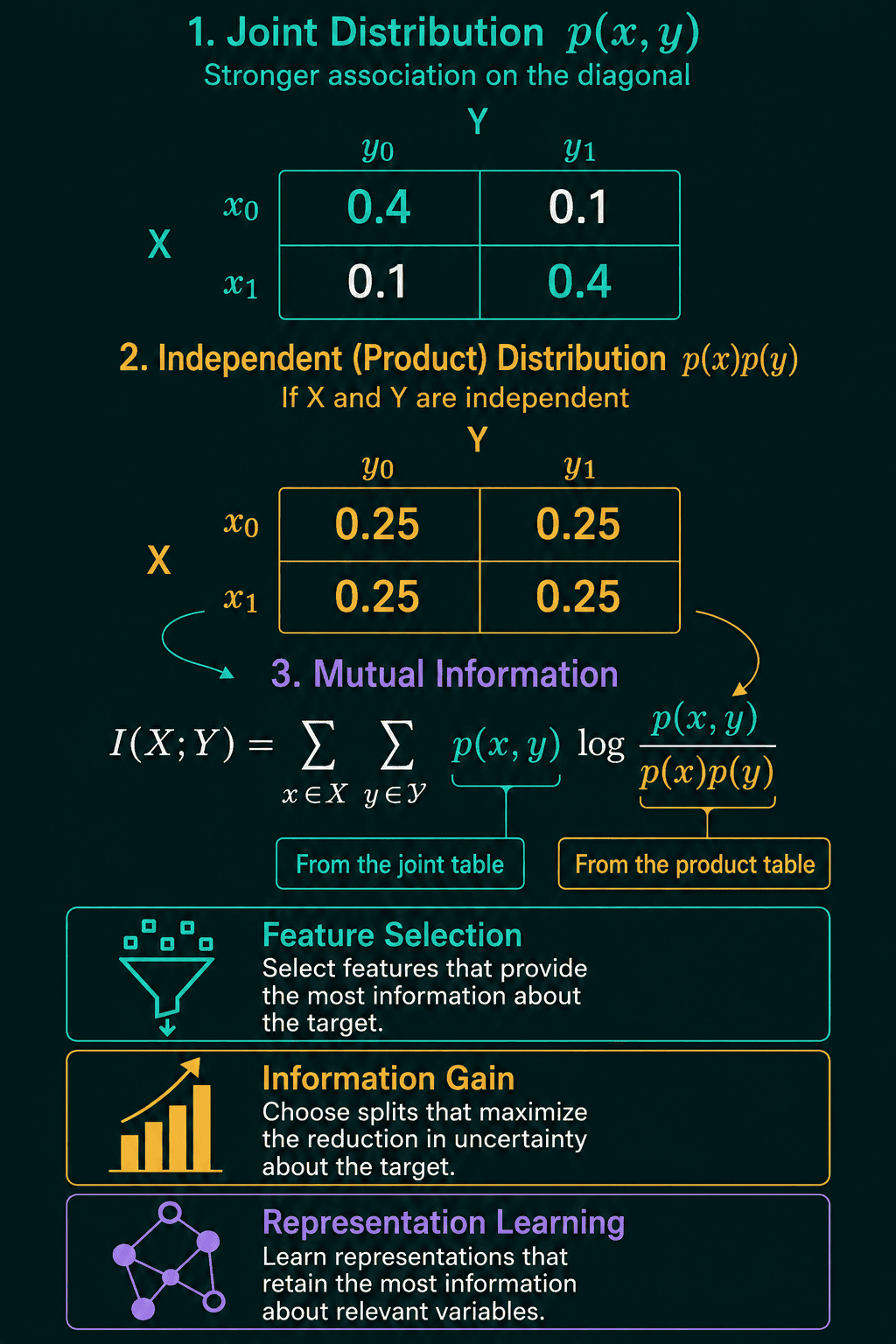
Feature selection. Ranking input features by their mutual information with the target keeps the ones that carry information about it, including relationships a correlation would miss.
Decision trees. The ID3 algorithm picks the split with the highest information gain, $H(\text{label}) - H(\text{label} \mid \text{feature})$, which is exactly $I(\text{feature}; \text{label})$. C4.5 divides that gain by how much the split fragments the data, which gives the gain ratio.
Representation learning. Some image models are trained on two altered copies of the same photo, for example a crop and a recolor, with an objective that pushes the two representations to share as much mutual information as possible.

The joint table p(x, y) and the independent product table p(x)p(y) feeding into the formula for I(X; Y), above three uses: feature selection, information gain for decision tree splits, and representation learning.

When to use it, and common mistakes

Use mutual information when you want to know whether two variables are related at all, in any shape. Correlation is enough when the question is only whether they move together along a straight line.

Using one conditional slice instead of the average. $H(Y \mid X)$ is the average of $H(Y \mid X{=}x)$ over all $x$, weighted by $p(x)$, not the entropy of a single row.
Dropping keepdim=True. The product of the marginals then comes out as a vector or a shape error instead of the (n, m) table.
Mixing units. torch.log gives nats. Divide by $\ln 2$ to compare with a value in bits, so 0.193 nats is about 0.278 bits.

What is entropy in information theory? covers entropy, the quantity mutual information is built from. Entropy, cross-entropy and KL divergence covers the KL divergence used in the second formula. Covariance vs correlation covers the linear measure that mutual information is often compared with.

QuiddityML teaches mutual information in the Math track's information theory unit. The exercises on it include filling in the joint entropy decomposition and writing mutual_information from the joint table and its independent version.