By Sagi Shaier · 17 October 2026 · 6 min read
Covariance vs correlation
How to compute covariance and correlation by hand and in PyTorch, why correlation is the one to compare across datasets, and how covariance decides whether the uncertainty of two quantities adds up or cancels.
Covariance and correlation both measure how two quantities move together: whether one tends to be high when the other is high, or low when the other is high. Covariance is the raw version, in the units of the data. Correlation is covariance rescaled to always land between $-1$ and 1, which makes it comparable across datasets. Both show up when looking for features that track a target, and covariance also decides how the uncertainty of a sum behaves.
A running example
Five students report how many hours they studied and the score they got:
| Student | Hours $x$ | Score $y$ |
|---|---|---|
| 1 | 1 | 52 |
| 2 | 2 | 58 |
| 3 | 3 | 57 |
| 4 | 4 | 66 |
| 5 | 5 | 72 |
The average is 3 hours and 61 points. More hours tend to go with a higher score, though student 3 scored a little lower than student 2.
Covariance
The variance of one quantity is the average squared distance from its mean. Covariance does the same for two quantities at once. For each pair, take how far $x$ is from its mean and how far $y$ is from its mean. Multiply the two distances and average the products:
$$\mathrm{Cov}(X,Y) = \mathbb{E}\big[(X - \mathbb{E}[X])(Y - \mathbb{E}[Y])\big]$$
$\mathbb{E}[\cdot]$ means "the average value of", so $\mathbb{E}[X]$ is the mean of $X$.
For the students, the distances of the hours from 3 are $-2, -1, 0, 1, 2$, and the distances of the scores from 61 are $-9, -3, -4, 5, 11$. The products are 18, 3, 0, 5 and 22. Their average is
$$\mathrm{Cov}(X,Y) = \frac{18 + 3 + 0 + 5 + 22}{5} = 9.6$$
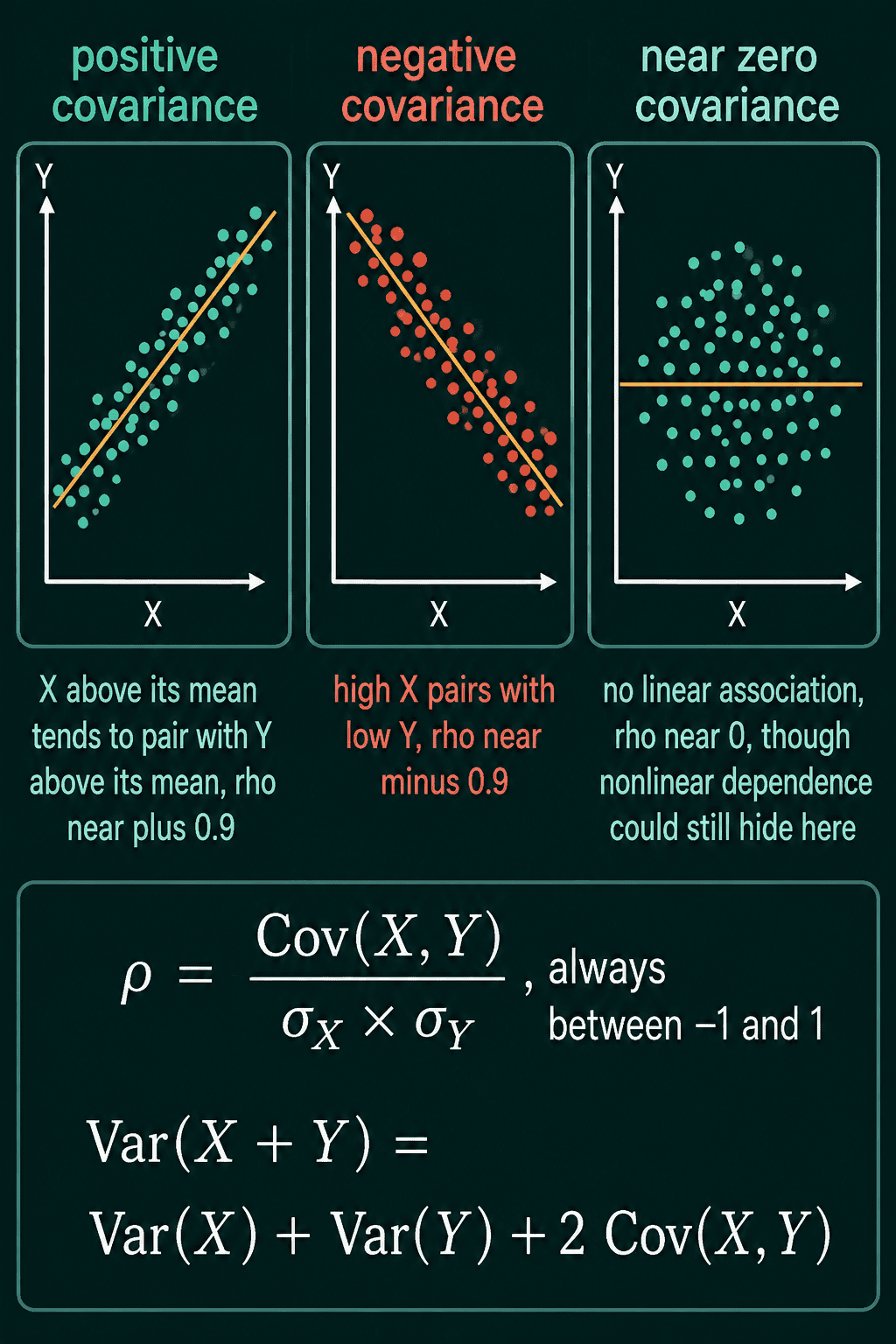
The sign of each product is what makes this work. A student above average on both, like student 5, gives a positive product. A student below average on both, like student 1, also gives a positive product because two negatives multiply to a positive. A student above average on one and below on the other gives a negative product. So:
- Positive covariance means the two tend to be above their means together and below their means together.
- Negative covariance means one tends to be high when the other is low.
- Covariance near zero means there is no linear co-movement, where linear means one tends to rise or fall along with the other at a steady rate.
The problem with covariance: units
Covariance carries the units of both quantities multiplied together. The 9.6 above is in hour-points. Measure study time in minutes instead and every hour distance is 60 times larger. The covariance becomes $9.6 \times 60 = 576$, even though nothing about the students changed. With house prices in dollars and floor area in square feet, the covariance is in dollar-feet. The raw size of a covariance is hard to read, and a covariance of 100 can be large or tiny depending on the scale of the variables.
Correlation
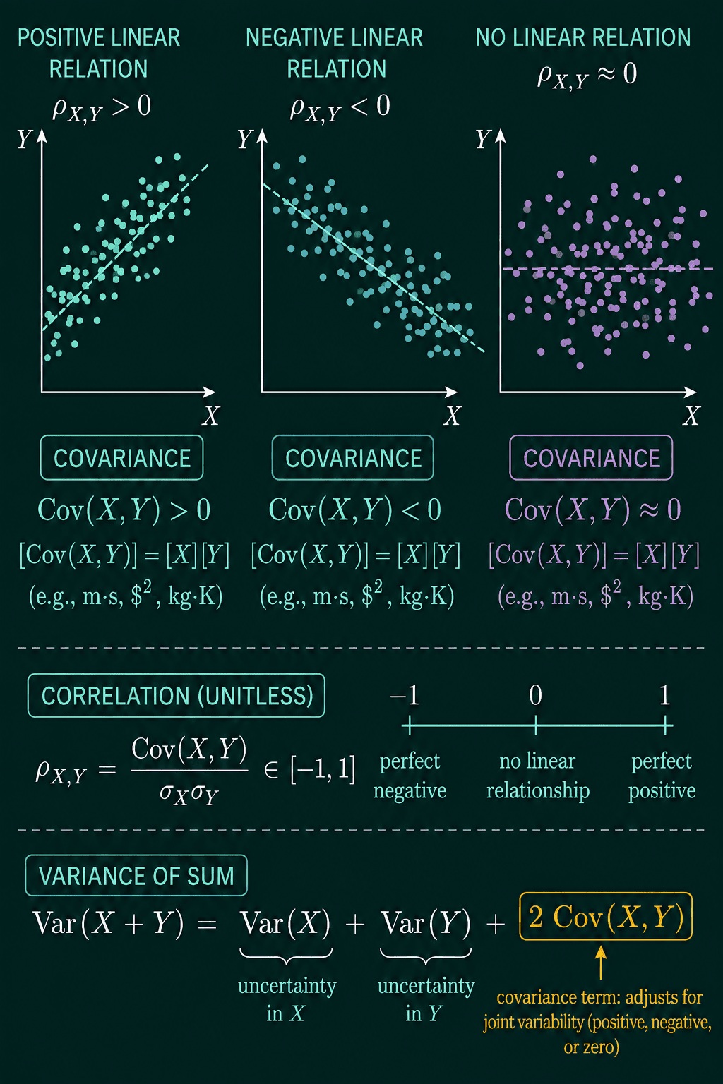
Correlation fixes the units by dividing the covariance by both standard deviations, where a standard deviation $\sigma$ (sigma) is the square root of the variance:
$$\rho_{XY} = \frac{\mathrm{Cov}(X,Y)}{\sigma_X\,\sigma_Y}$$
$\rho$ (rho) is the usual symbol for correlation. For the students, the hours have variance 2 and the scores have variance 50.4, so $\sigma_X = 1.414$ and $\sigma_Y = 7.099$. Then
$$\rho_{XY} = \frac{9.6}{1.414 \times 7.099} = 0.956$$
Switching to minutes multiplies the covariance by 60 and $\sigma_X$ by 60 too, so the two cancel and the correlation stays 0.956. Correlation always lands between $-1$ and 1:
- near 1: a strong positive linear relationship, the points sit close to a rising line
- near $-1$: a strong negative linear relationship, close to a falling line
- near 0: little linear relationship
Covariance and correlation in PyTorch
For paired samples stored as two tensors, covariance is one line. x.std(unbiased=False) gives the standard deviation with the same $1/n$ average that .mean() uses:
1import torch
2
3hours = torch.tensor([1.0, 2.0, 3.0, 4.0, 5.0])
4score = torch.tensor([52.0, 58.0, 57.0, 66.0, 72.0])
5
6def covariance(x, y):
7    return ((x - x.mean()) * (y - y.mean())).mean()
8
9def correlation(x, y):
10    return covariance(x, y) / (x.std(unbiased=False) * y.std(unbiased=False))
11
12print(covariance(hours, score), correlation(hours, score))
13minutes = hours * 60
14print(covariance(minutes, score), correlation(minutes, score))
15print(torch.corrcoef(torch.stack([hours, score]))[0, 1])
16# tensor(9.6000) tensor(0.9562)
17# tensor(576.) tensor(0.9562)
18# tensor(0.9562)
The second line shows the units problem: the covariance jumps from 9.6 to 576 and the correlation does not move. torch.corrcoef computes the same correlation for every pair of rows in a stacked tensor.
Zero correlation does not mean unrelated
Covariance and correlation only measure the linear part of a relationship. Take $x$ values of $-2, -1, 0, 1, 2$ and set $y = x^2$. Each $y$ is fully decided by its $x$, and the covariance is still exactly 0:
1import torch
2
3x = torch.tensor([-2.0, -1.0, 0.0, 1.0, 2.0])
4y = x ** 2
5cov = ((x - x.mean()) * (y - y.mean())).mean()
6print(y, cov)
7# tensor([4., 1., 0., 1., 4.]) tensor(0.)
The left half of the points falls and the right half rises, and the two halves cancel. A correlation near 0 rules out a straight-line relationship and nothing more, so a scatter plot is worth a look before concluding that two quantities are unrelated.
Covariance in the variance of a sum
Covariance also controls how uncertainty adds. For any two random quantities:
$$\mathrm{Var}(X+Y) = \mathrm{Var}(X) + \mathrm{Var}(Y)$$
$$+\, 2\,\mathrm{Cov}(X,Y)$$
If $X$ and $Y$ are independent, meaning knowing one tells you nothing about the other, their covariance is 0 and the variances add. If they move together, the sum varies more than the two variances suggest. If they move in opposite directions, some of the variation cancels. A simulation shows both cases, with two quantities that each have variance 1:
1import torch
2
3torch.manual_seed(0)
4n = 100_000
5x = torch.randn(n)
6noise = torch.randn(n)
7y_same = 0.8 * x + 0.6 * noise      # moves with x
8y_opp = -0.8 * x + 0.6 * noise      # moves against x
9
10for name, y in (("together", y_same), ("opposite", y_opp)):
11    cov = ((x - x.mean()) * (y - y.mean())).mean()
12    print(name, round(x.var().item(), 2), round(y.var().item(), 2), round(cov.item(), 2), round((x + y).var().item(), 2))
13# together 1.0 1.0 0.8 3.6
14# opposite 1.0 1.01 -0.81 0.4
Moving together, the sum has variance $1 + 1 + 2(0.8) = 3.6$. Moving in opposite directions, it has $1 + 1 - 2(0.8) = 0.4$, less than either one alone.
The same formula explains why averaging many estimates helps most when their errors do not all move together. Errors with positive covariance add up instead of cancelling, so an average of five models that make the same mistakes is not much better than one of them.
Common mistakes
- Mixing the $n$ and $n - 1$ divisors. PyTorch's
x.std()divides by $n - 1$ by default, while the covariance above divides by $n$. Mixing the two gives a wrong correlation, shown in the snippet after this list. - Comparing raw covariances across datasets. A covariance of 576 is not a stronger relationship than 9.6. It is the same data in minutes, so compare correlations.
- Reading zero correlation as independence. Independence gives zero covariance, but zero covariance does not give independence, as $y = x^2$ shows.
- Reading correlation as cause. A correlation of 0.956 between hours and score says the two rise together. It does not say which one drives the other, or whether something else drives both.
The divisor mix-up gives 0.765 instead of 0.956 on the student data:
1import torch
2
3hours = torch.tensor([1.0, 2.0, 3.0, 4.0, 5.0])
4score = torch.tensor([52.0, 58.0, 57.0, 66.0, 72.0])
5cov = ((hours - hours.mean()) * (score - score.mean())).mean()
6print(cov / (hours.std() * score.std()))                                  # std divides by n - 1
7print(cov / (hours.std(unbiased=False) * score.std(unbiased=False)))      # std divides by n
8# tensor(0.7649)
9# tensor(0.9562)
Related concepts
Expected value and variance covers the variance that covariance generalizes. Degrees of freedom explains when to divide by $n - 1$ instead of $n$. The multivariate Gaussian collects the variances and covariances of many quantities into one covariance matrix. Joint, marginal and conditional probability defines independence, the case where the covariance term drops out.
QuiddityML teaches covariance and correlation as a concept in the Math track's probability unit, and the exercises on it include filling in the variance-of-a-sum identity, ordering the lines of covariance and correlation and writing both functions from scratch with the $n$ divisor.