By Sagi Shaier · 22 October 2026 · 4 min read
Exponential moving average (EMA) explained
How the EMA update works, why it starts too low and how bias correction fixes that, and how to read a beta like 0.9 or 0.999 as a window.
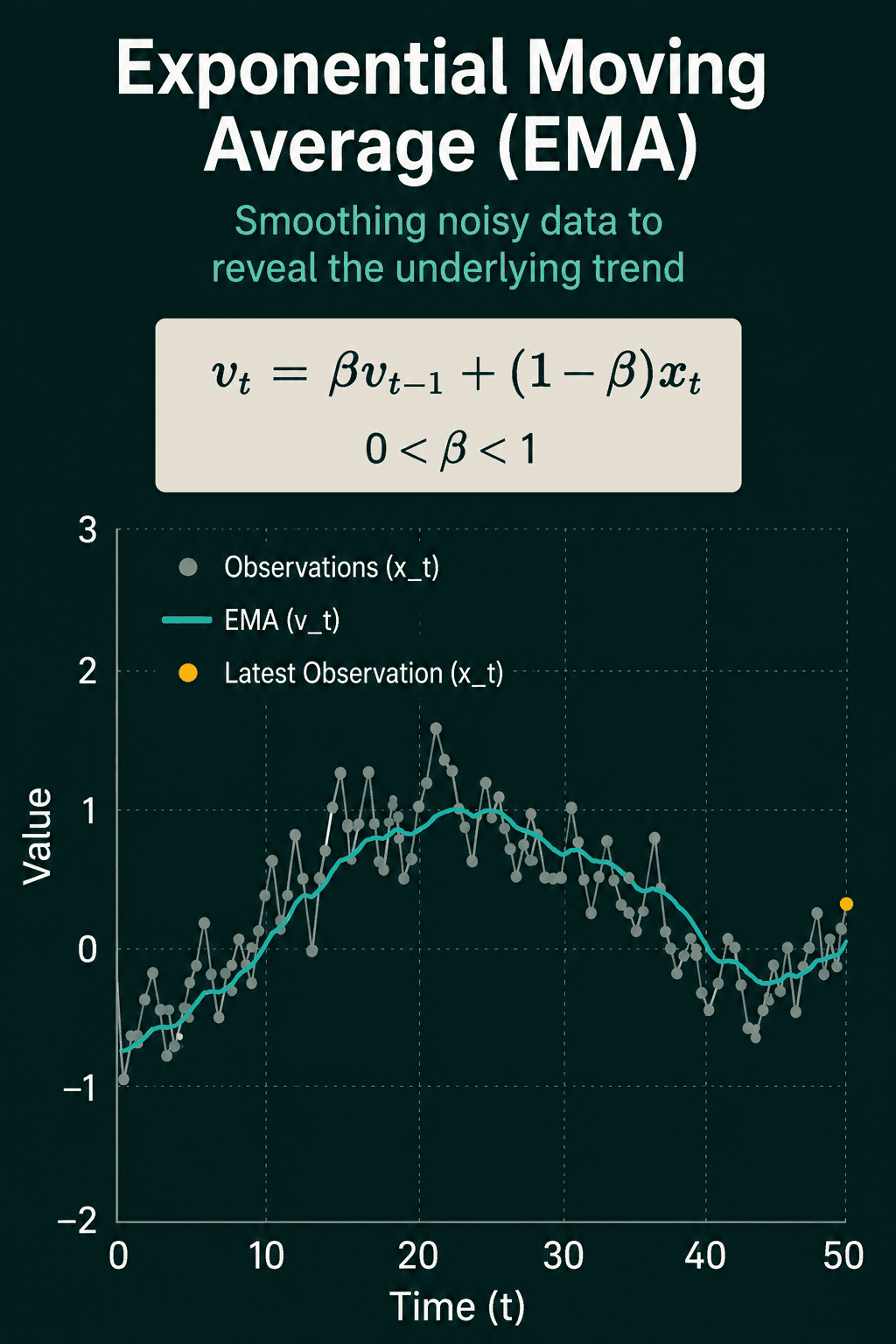
An exponential moving average (EMA) is a running average that gives the newest value the most weight and lets older values fade out gradually, without storing the history. It is a common way to smooth a noisy stream of numbers, like sensor readings or daily temperatures, so the overall level shows through the jumps.
What problem does an EMA solve?
Sensor readings, daily temperatures and website traffic all jump around from one reading to the next. A smoothed estimate that follows the overall level, nudged a little with every new reading, is often more useful than any single noisy value.
A plain average would treat every value equally and needs either the full list or a count of how many values came before. An EMA keeps one number and updates it in place, weighting recent values more than old ones.
The EMA update rule
Call the running average after step $t$ by the name $v_t$, and the newest observed value $x_t$. A number $\beta$ between 0 and 1, usually close to 1, sets how much of the old average is kept. The update is
$$v_t = \beta v_{t-1} + (1 - \beta) x_t$$
The new average is a blend: a $\beta$ share of the old average plus a $(1 - \beta)$ share of the newest value. A high $\beta$ like 0.99 moves slowly and smooths out noise. A low $\beta$ like 0.5 reacts quickly and smooths less.
A worked example
Take $\beta = 0.9$, start from $v_0 = 0$, and feed in the value 10 three times:
$$v_1 = 0.9 \times 0 + 0.1 \times 10 = 1.0$$
$$v_2 = 0.9 \times 1.0 + 0.1 \times 10 = 1.9$$
$$v_3 = 0.9 \times 1.9 + 0.1 \times 10 = 2.71$$
The average climbs toward 10, slowly. In code the update is one line inside a loop:
1def ema(values, beta):
2    v, out = 0.0, []
3    for x in values:
4        v = beta * v + (1 - beta) * x
5        out.append(round(v, 4))
6    return out
7
8print(ema([10, 10, 10], beta=0.9))
9# [1.0, 1.9, 2.71]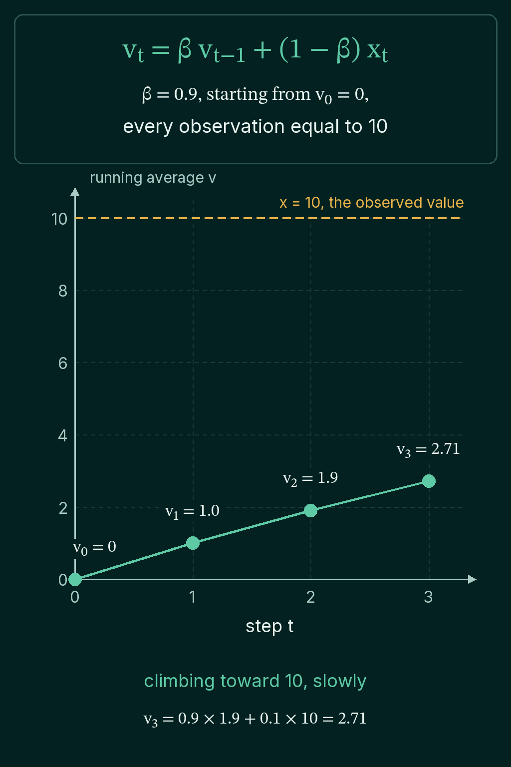
Unrolling the recurrence
Each $v_t$ is built from $v_{t-1}$, which is built from $v_{t-2}$, and so on. Substituting each one into the next, all the way down to $v_0 = 0$, turns the update into a weighted sum over every value seen so far:
$$v_t = (1 - \beta) \sum_{k=0}^{t-1} \beta^k x_{t-k}$$
Here $k$ counts how many steps back a value is, so $x_{t-k}$ is the value from $k$ steps ago and its weight is $(1 - \beta)\beta^k$. With $\beta = 0.9$ the newest value gets weight 0.1 and the one before it gets 0.09. After that come 0.081 and 0.0729, each weight 0.9 times the one before.
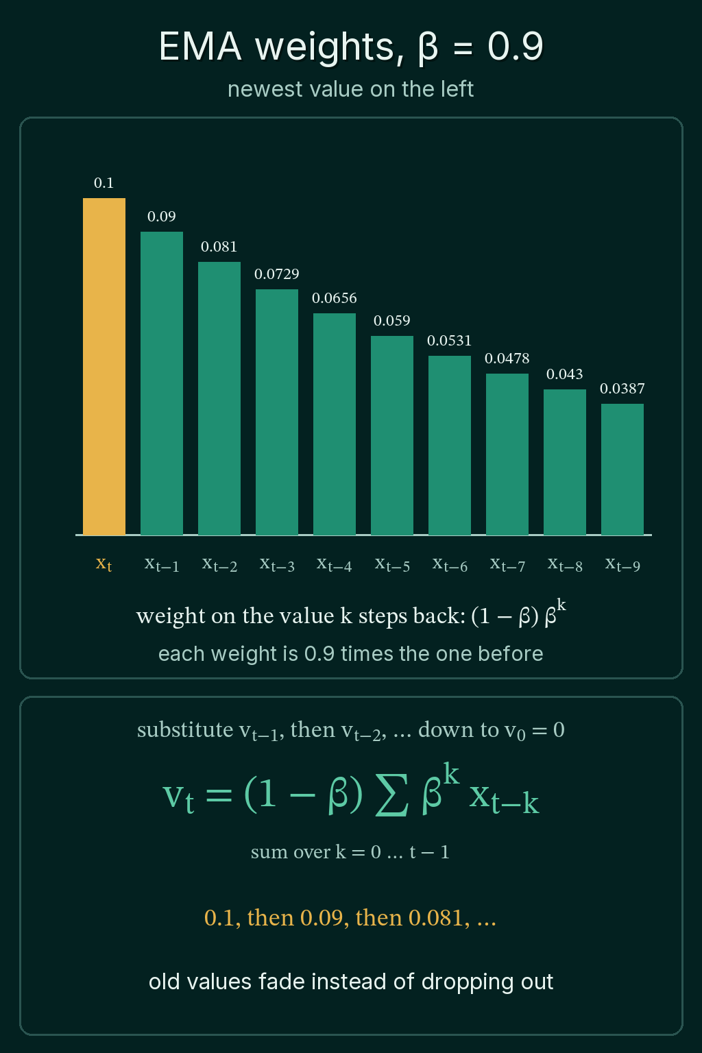
Every past value is still in the average. Its weight shrinks by the same factor at each step back, which is where the word "exponential" comes from.
Bias correction
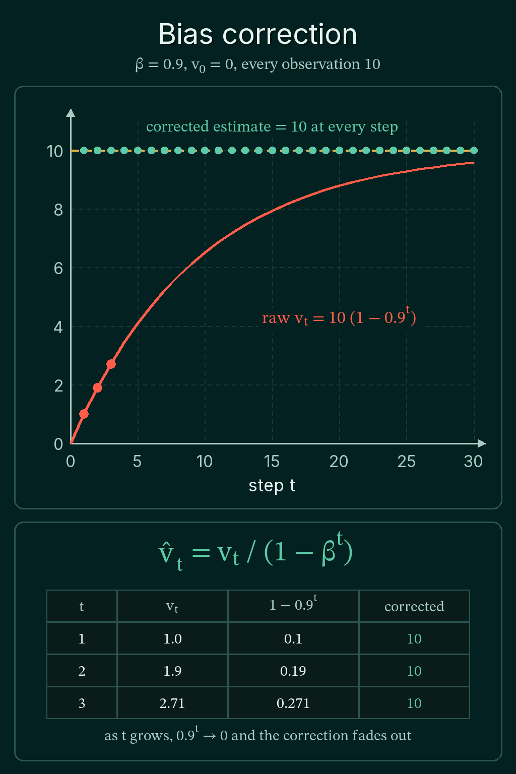
An EMA that starts at $v_0 = 0$ begins too low. After three observations of 10, the worked example still reads 2.71, which is a poor estimate of a stream that has been 10 the whole time. The weights explain why: after $t$ steps they add up to $1 - \beta^t$ instead of 1, and the missing share still belongs to the starting value of 0.
Bias correction divides that missing share back out. The corrected estimate, written $\hat v_t$, is
$$\hat v_t = \frac{v_t}{1 - \beta^t}$$
At $t = 1$ with $\beta = 0.9$ the divisor is $1 - 0.9 = 0.1$, so $\hat v_1 = 1.0 / 0.1 = 10$. At $t = 2$ it is $1 - 0.81 = 0.19$, and $1.9 / 0.19 = 10$ again. As $t$ grows, $\beta^t$ shrinks toward 0 and the divisor approaches 1, so the correction fades out once the EMA has seen enough values.
1def ema_corrected(values, beta):
2    v, out = 0.0, []
3    for t, x in enumerate(values, start=1):
4        v = beta * v + (1 - beta) * x
5        out.append(round(v / (1 - beta ** t), 4))
6    return out
7
8print(ema_corrected([10, 10, 10], beta=0.9))
9print(ema_corrected([10, 12, 8, 30, 10, 10], beta=0.9))
10# [10.0, 10.0, 10.0]
11# [10.0, 11.0526, 9.9262, 15.7633, 14.3559, 13.4263]
The second stream has a spike to 30 at step 4. The corrected average moves up to about 15.8 and then eases back down, since the spike keeps a shrinking share of the weight.
Reading beta as a window
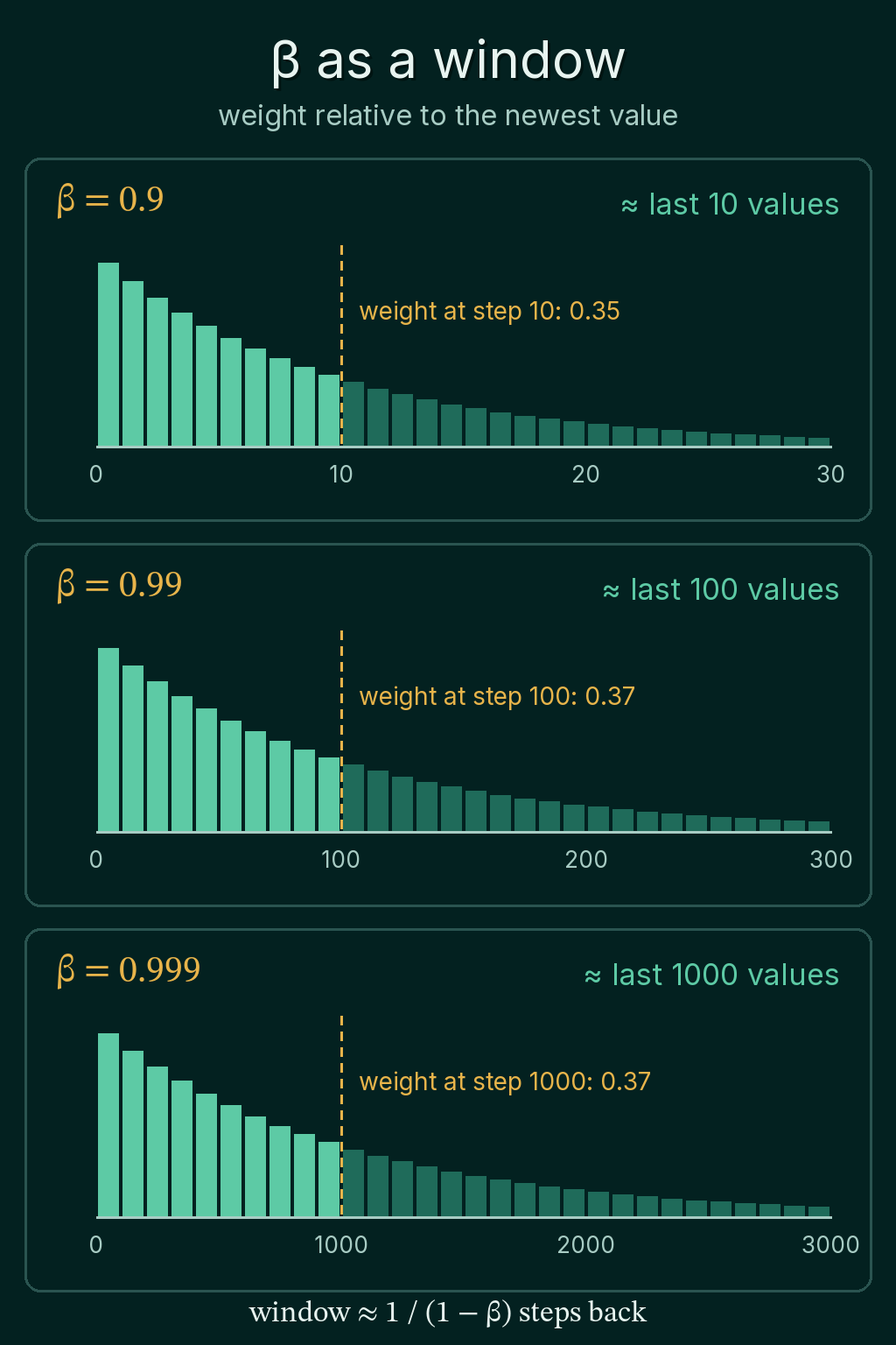
A quick way to read a $\beta$ is as a window: an EMA averages over roughly the last $1 / (1 - \beta)$ values. So $\beta = 0.9$ covers about the last 10 values, $\beta = 0.99$ about the last 100, and $\beta = 0.999$ about the last 1000.
The window has no hard edge. At the window's end, the weight on a value is still about 35% to 37% of the weight on the newest value, and older values keep a smaller share after that.
Common mistakes
- Skipping bias correction for early values. An EMA started at 0 reads low for roughly the first $1 / (1 - \beta)$ steps. Correct it if those early values get used.
- Applying bias correction to an EMA that did not start at 0. If $v_0$ is set to the first observation, the estimate is not biased toward 0 and dividing by $1 - \beta^t$ makes it too high.
- Choosing $\beta$ without thinking about the window. $\beta = 0.999$ reacts to a change only after hundreds of values.
Related concepts
Expected value and variance covers the plain average an EMA is compared against. The Adam optimizer and machine learning optimizers show where running averages like this one appear in training.
QuiddityML teaches the exponential moving average as a concept in the Math track's numerical computation unit. The exercises on it include turning the update rule into an ema_step function, picking the line that bias-corrects an EMA, and spotting the bug in an EMA loop.