26 September 2026 · 8 min read

Entropy, cross-entropy, and KL divergence explained

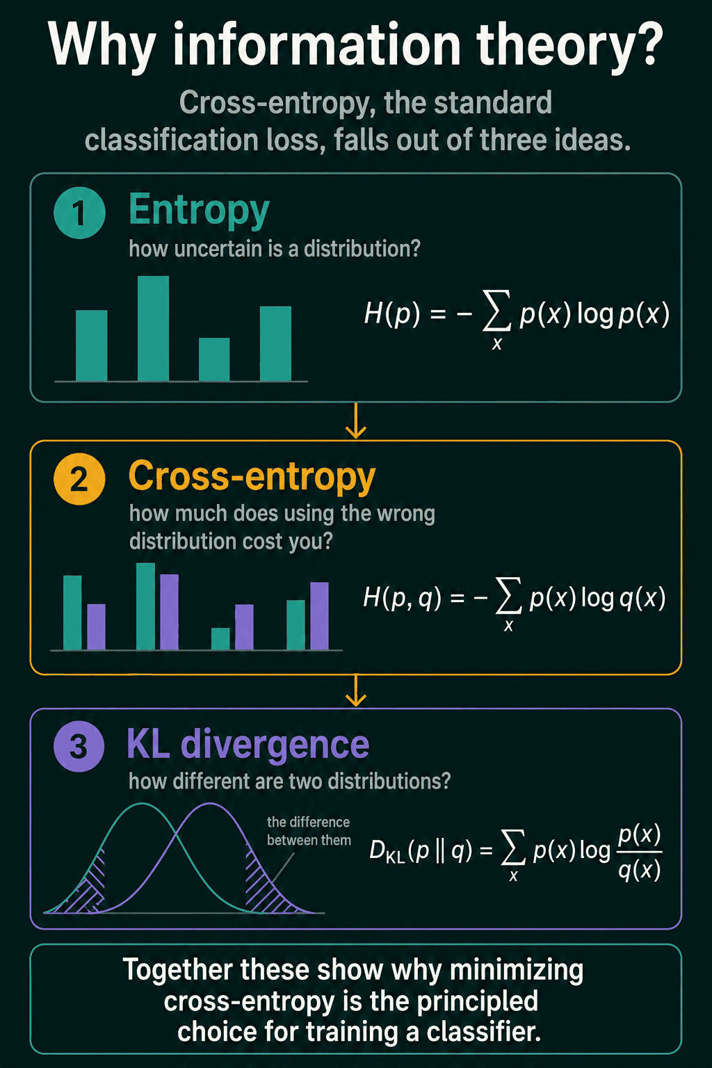
Cross-entropy is the usual loss for training a classifier. This post explains where it comes from, starting with entropy and ending with KL divergence, works each one out on the same small example, and shows how to compute them in PyTorch.

Cross-entropy loss is the negative log of the probability a model gave to the correct answer. A classifier that puts 0.9 on the right class gets a small loss, and one that puts 0.1 on it gets a large one. It is the usual loss for image classifiers, text classifiers, and language models predicting the next word. The formula comes from information theory, and it makes more sense next to the two quantities on either side of it: entropy and KL divergence.

What problem does cross-entropy solve?

A classifier outputs a probability for each class, such as cat 0.7, dog 0.2, bird 0.1. Training needs a loss that turns those probabilities and the correct label into one number, small when the model is right and confident, large when it is confidently wrong. Mean squared error trains poorly on probabilities, as the loss function post shows. Information theory builds a better loss in three steps:

Entropy: how uncertain one distribution is.
Cross-entropy: what it costs to use the wrong distribution.
KL divergence: how far apart two distributions are.

Entropy: how uncertain a distribution is

A probability distribution is a list of outcomes with a probability for each, adding up to 1. A fair coin is heads 0.5, tails 0.5, and the classifier output above is a distribution over three classes.

The surprise of an outcome $x$ with probability $p(x)$ is $-\log p(x)$. An outcome with probability 1 has surprise 0, and the rarer the outcome, the larger its surprise. With base-2 logs the unit is bits: probability 0.5 is 1 bit of surprise, 0.25 is 2 bits, 0.1 is 3.32 bits. In information theory, $-\log_2 p(x)$ is also the length of the code an efficient encoder built for $p$ spends on outcome $x$, so common outcomes get short codes and rare ones get long codes.

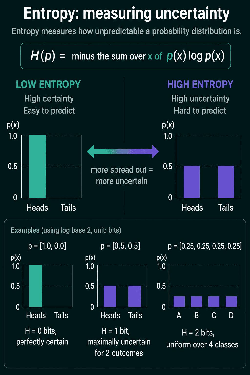
Entropy is the average surprise, where each outcome's surprise is weighted by how often it happens. For a distribution $p$ over outcomes $x$, entropy $H(p)$ is:

$$H(p) = -\sum_x p(x) \log p(x)$$

Low entropy means the probability is piled on a few outcomes, so the next outcome is easy to predict. High entropy means it is spread out. Three examples in bits:

$p = [1.0, 0.0]$: $H = 0$ bits. The outcome is certain.
$p = [0.5, 0.5]$: $H = 1$ bit, the most uncertain two outcomes can be.
$p = [0.25, 0.25, 0.25, 0.25]$: $H = 2$ bits, spread evenly over four outcomes.

Entropy of three distributions in bits: a certain coin at 0 bits, a fair coin at 1 bit, and a uniform distribution over four classes at 2 bits

Machine learning code uses the natural log, so PyTorch reports nats instead of bits, and the fair coin comes out as $\ln 2 \approx 0.693$ nats with the same math. On a classifier, entropy measures confidence: an output of $[0.99, 0.005, 0.005]$ has entropy 0.063 nats, and $[0.34, 0.33, 0.33]$ has 1.099 nats, almost the maximum of $\ln 3 \approx 1.0986$ for three classes.

Cross-entropy: the cost of using the wrong distribution

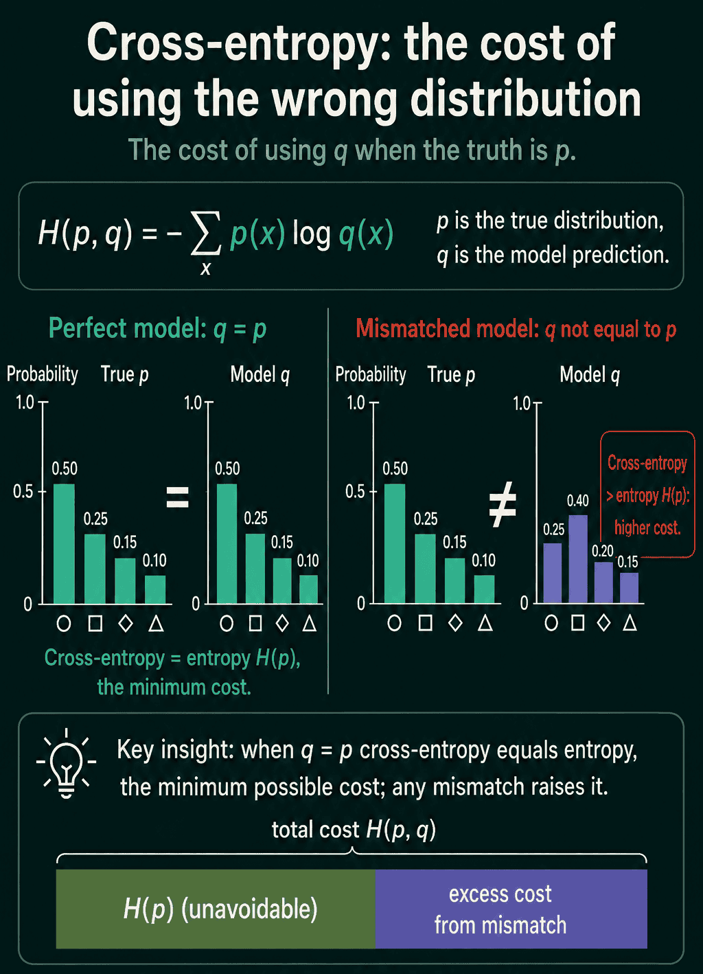
Training compares two distributions: the true distribution $p$, which comes from the label, and the model's prediction $q$. Cross-entropy $H(p, q)$ keeps the weights from $p$ but takes the surprise from $q$:

$$H(p, q) = -\sum_x p(x) \log q(x)$$

In coding terms, it is the average code length when outcomes come from $p$ but the codes were built for $q$. If $q = p$, cross-entropy equals the entropy $H(p)$, and that is the lowest it can go. Any mismatch between $q$ and $p$ raises it.

Take four classes with true distribution $p = [0.50, 0.25, 0.15, 0.10]$ and a model that predicts $q = [0.25, 0.40, 0.20, 0.15]$. The entropy of $p$ is 1.208 nats. The cross-entropy is:

$$H(p, q) = -(0.5 \ln 0.25 + 0.25 \ln 0.4$$

$$+, 0.15 \ln 0.2 + 0.1 \ln 0.15)$$

$$\approx 1.353 \text{ nats}$$

The 1.208 is the part no model can remove, because it is the uncertainty in $p$ itself. The extra 0.145 comes from the model predicting $q$ instead of $p$.

Cross-entropy for a perfect model where q equals p, which gives the minimum cost H(p), and for a mismatched model where q is 0.25, 0.40, 0.20, 0.15, which costs more, and the total splits into H(p) plus the excess cost from the mismatch

Cross-entropy with a one-hot label

In ordinary classification the label is one class. For a cat photo with classes cat, dog, bird, the true distribution is $p = [1, 0, 0]$, a vector with one 1 and zeros elsewhere, called one-hot. The terms with $p(x) = 0$ drop out of the sum, so cross-entropy becomes the negative log of the probability the model put on the correct class:

$$H(p, q) = -\log q(\text{correct class})$$

For $q = [0.7, 0.2, 0.1]$ the loss is $-\ln 0.7 \approx 0.357$. For $q = [0.99, 0.005, 0.005]$ it is 0.010. If the model had put 0.1 on cat, it would be 2.303. The entropy of a one-hot label is 0, so the loss can get down to 0 when the model puts probability 1 on the right class.

Averaged over a batch, this is the loss classifiers train on. The model produces raw scores and softmax turns them into $q$. Binary cross-entropy is the two-class case, with $p = [y, 1 - y]$ for a label $y$ of 0 or 1.

KL divergence: the gap between cross-entropy and entropy

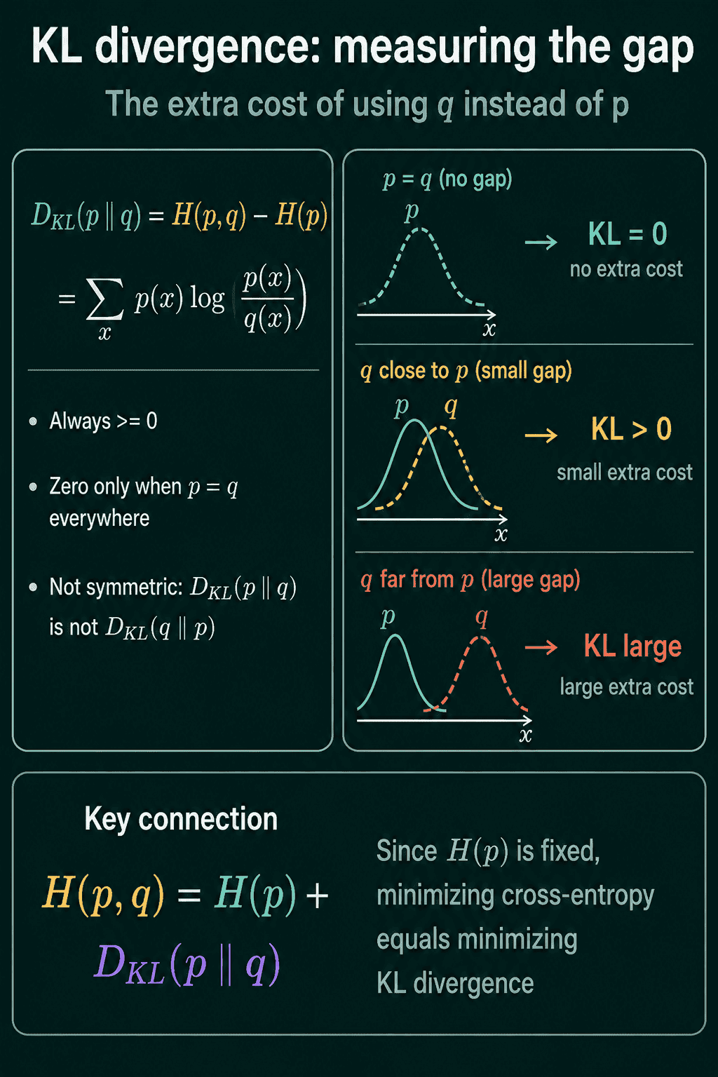
Kullback-Leibler (KL) divergence is the extra cost from the mismatch, cross-entropy minus entropy:

$$D_{\text{KL}}(p ,|, q) = H(p, q) - H(p)$$

$$= \sum_x p(x) \log \frac{p(x)}{q(x)}$$

For the four-class example, $1.353 - 1.208 = 0.145$ nats. Three properties follow from the math:

It is never negative, because cross-entropy never drops below entropy.
It is 0 exactly when $q = p$.
It is not symmetric. Swapping the two gives $D_{\text{KL}}(q ,|, p) \approx 0.133$ for the same example. The gap can be much larger: with $p = [0.5, 0.5]$ and $q = [1, 0]$, $D_{\text{KL}}(p ,|, q)$ is infinite, because $p$ puts probability on an outcome $q$ calls impossible, while $D_{\text{KL}}(q ,|, p) = \ln 2 \approx 0.693$. This is why KL divergence is not a distance.

Rearranged, the definition says $H(p, q) = H(p) + D_{\text{KL}}(p ,|, q)$. The labels fix $p$, so $H(p)$ is a constant during training, and minimizing cross-entropy and minimizing KL divergence change the weights in exactly the same way. Cross-entropy is used because it is the part you compute directly from the label and the prediction. With one-hot labels $H(p) = 0$, so the two numbers are equal.

KL divergence equals cross-entropy minus entropy, is at least 0, is 0 only when p equals q, grows as q moves away from p, and is not symmetric, and since H(p) is fixed, minimizing cross-entropy equals minimizing KL divergence

KL divergence is used directly when neither distribution is a hard label. In knowledge distillation, a small student model is trained to match the probability distribution of a larger teacher model, with KL divergence as the loss. Variational autoencoders use it to measure how far a learned distribution over hidden variables drifts from a fixed prior distribution.

Entropy measures how uncertain one distribution is, cross-entropy measures the cost of using the wrong distribution, and KL divergence measures the difference between two distributions, which together show why classifiers train by minimizing cross-entropy

Entropy, cross-entropy, and KL divergence in PyTorch

Each one is a line of tensor operations. This checks them on the four-class example and against PyTorch's built-in functions:

1import torch
2import torch.nn.functional as F
3 
4def entropy(p):
5    return -(p * torch.log(p)).sum()
6 
7def cross_entropy(p, q):
8    return -(p * torch.log(q)).sum()
9 
10def kl_divergence(p, q):
11    return (p * torch.log(p / q)).sum()
12 
13p = torch.tensor([0.50, 0.25, 0.15, 0.10])   # true distribution
14q = torch.tensor([0.25, 0.40, 0.20, 0.15])   # model's prediction
15 
16print(entropy(p))            # 1.2080
17print(cross_entropy(p, q))   # 1.3533
18print(kl_divergence(p, q))   # 0.1454, the gap between the two lines above
19print(kl_divergence(q, p))   # 0.1331, a different number with p and q swapped
20 
21# F.cross_entropy takes logits, and log(q) works as logits because softmax(log q) = q.
22print(F.cross_entropy(torch.log(q).unsqueeze(0), p.unsqueeze(0)))  # 1.3533
23# F.kl_div takes the model's log-probabilities first and the target second.
24print(F.kl_div(torch.log(q), p, reduction="sum"))                   # 0.1454

In a real model you pass raw logits and class indices to nn.CrossEntropyLoss, which applies log-softmax itself. For distillation, compare log-probabilities from the student with probabilities from the teacher:

1import torch
2import torch.nn as nn
3import torch.nn.functional as F
4 
5torch.manual_seed(0)
6logits = torch.randn(8, 3)                # a batch of 8 examples, 3 classes
7targets = torch.randint(0, 3, (8,))       # correct class index for each example
8 
9loss = nn.CrossEntropyLoss()(logits, targets)
10manual = -F.log_softmax(logits, dim=1)[torch.arange(8), targets].mean()
11print(loss, manual)                       # the same number
12 
13teacher_logits = torch.randn(8, 3)
14student_logits = torch.randn(8, 3, requires_grad=True)
15kl = F.kl_div(
16    F.log_softmax(student_logits, dim=1),   # input: student log-probabilities
17    F.softmax(teacher_logits, dim=1),       # target: teacher probabilities
18    reduction="batchmean",                  # sum over classes, mean over examples
19)
20kl.backward()

If the loss comes out as nan or inf, check first for a probability of exactly 0 going into a hand-written torch.log.

When to use each one

Cross-entropy is the loss to reach for in classification with labels, including next-word prediction in language models. Use nn.CrossEntropyLoss for one class per example and nn.BCEWithLogitsLoss for yes/no labels.
KL divergence is the loss when the target is itself a model's distribution, such as a teacher in distillation or a prior in a variational autoencoder.
Entropy is more often a measure than a loss, for example to flag inputs where the model's prediction is spread out.

Common mistakes

Taking the log of a zero probability. torch.log(0) is -inf, and 0 * -inf is nan, so entropy(torch.tensor([0.5, 0.5, 0.0])) returns nan with no error. Work from logits with F.log_softmax or the built-in losses, which avoid computing log(0).
Swapping the arguments to F.kl_div. The first argument is the model's log-probabilities and the second is the target's probabilities. Passing plain probabilities as the first argument gives a wrong number and no error.
Using reduction="mean" with F.kl_div. It divides by the number of classes as well as the batch size. On the four-class example it returns 0.0363, a quarter of 0.1454, and PyTorch prints a warning. Use "batchmean".
Flipping the KL direction. $D_{\text{KL}}(p ,|, q)$ and $D_{\text{KL}}(q ,|, p)$ are different numbers that push a model toward different fits.
Expecting cross-entropy to reach 0 with soft targets. The floor is $H(p)$, which is 0 only for one-hot labels. With label_smoothing=0.1 over 10 classes the target puts 0.91 on the correct class and 0.01 on each other one, so the lowest possible loss is about 0.500.

The loss function post covers softmax, binary cross-entropy, their PyTorch classes, and when to pick a different loss. Maximum likelihood estimation gives a second route to the same loss: making the correct labels as probable as possible under the model is the same as minimizing cross-entropy. Perplexity, the number often reported for language models, is $e$ raised to the average cross-entropy per token. Backpropagation computes the gradient of the loss for each weight, and gradient descent uses it to lower the loss.

QuiddityML teaches information theory, entropy, cross-entropy, and KL divergence as four short concepts in the first unit of its ML Foundation track, and the exercises include writing each formula in PyTorch from scratch, spotting the missing minus sign in an entropy function, predicting the nan that log(0) produces, and picking the assertion that checks KL divergence equals cross-entropy minus entropy.