By Sagi Shaier · 21 October 2026 · 9 min read
What is entropy in information theory?
How to compute entropy by hand and in PyTorch, what bits and nats are, why it can go negative for continuous variables and how the maximum entropy principle picks a distribution from a few known facts.
Entropy is a single number that says how unpredictable a probability distribution is: low when one outcome is almost certain, high when many outcomes are about equally likely. It comes up wherever a model outputs probabilities. Classification losses are built from it, and decision trees use it to choose their splits.
Self-information: how surprising is one outcome?
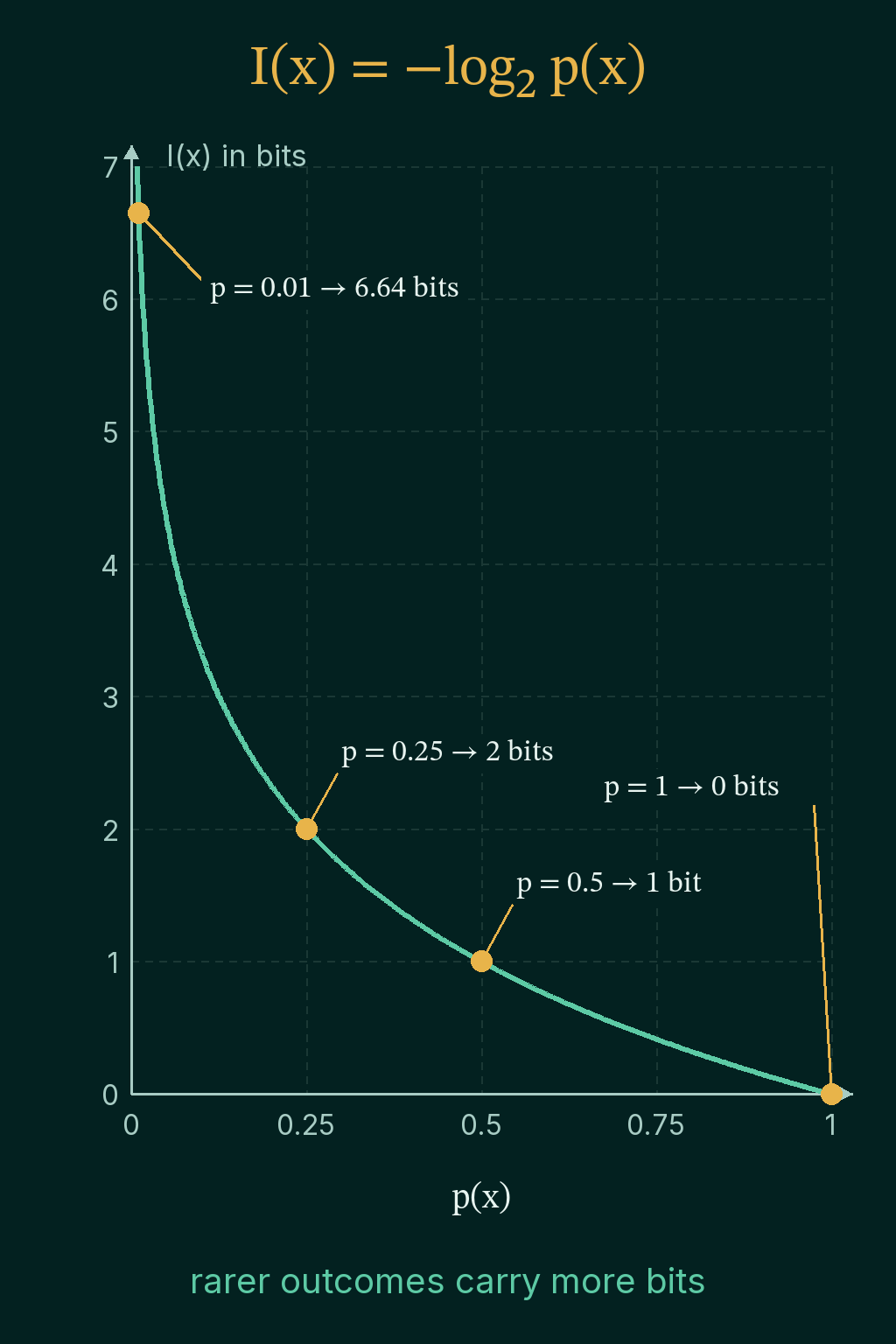
Entropy is built from a smaller quantity that measures one outcome at a time. Take a coin that lands heads 99% of the time. Heads tells you almost nothing new, and tails at 1% is a real surprise. Self-information, also called surprisal, puts a number on that surprise. For an outcome $x$ with probability $p(x)$:
$$I(x) = -\log p(x)$$
The log of a probability is zero or negative, because a probability is a number from 0 to 1, and the minus sign flips it so surprisal comes out zero or positive. With $\log_2$, the log in base 2, the unit is the bit. A few values to check by hand:
- $p(x) = 1$ gives $I(x) = -\log_2 1 = 0$ bits. A certain outcome carries no surprise.
- $p(x) = 0.5$ gives $-\log_2 0.5 = 1$ bit, the surprise of a fair coin flip.
- $p(x) = 0.25$ gives $-\log_2 0.25 = 2$ bits, since $0.25 = 2^{-2}$.
- $p(x) = 0.01$ gives $-\log_2 0.01 \approx 6.64$ bits.
As $p(x)$ heads toward 0, the surprisal grows without limit, so rare outcomes carry the most information when they happen.
Entropy: the average surprise of a distribution
A probability distribution lists every outcome with its probability, and the probabilities add up to 1. A fair coin is heads 0.5, tails 0.5. A forecast of sun 0.7, cloud 0.2 and rain 0.1 is also a distribution.
Entropy is the surprisal of each outcome, averaged with each outcome weighted by how often it happens:
$$H(p) = \sum_x p(x)\, I(x) = -\sum_x p(x) \log p(x)$$
$H(p)$ is the entropy of the distribution $p$, and the sum runs over every outcome $x$. For the fair coin, each outcome has surprisal 1 bit and probability 0.5:
$$H = 0.5 \cdot 1 + 0.5 \cdot 1 = 1 \text{ bit}$$
For the 99/1 coin, heads has surprisal $-\log_2 0.99 \approx 0.0145$ bits and tails has 6.64 bits:
$$H \approx 0.99 \cdot 0.0145 + 0.01 \cdot 6.64 \approx 0.081 \text{ bits}$$
Tails is very surprising, but it happens so rarely that the average stays close to 0. That is what low entropy means: the distribution is concentrated, so its outcomes are easy to predict. High entropy means it is spread out.
Two more examples. A distribution with $p = [1.0, 0.0]$ has entropy 0. The term for the impossible outcome is $0 \log 0$, which is taken to be 0 because $p \log p$ shrinks to 0 as $p$ shrinks to 0. Four equally likely outcomes, $p = [0.25, 0.25, 0.25, 0.25]$, give $4 \cdot 0.25 \cdot 2 = 2$ bits.
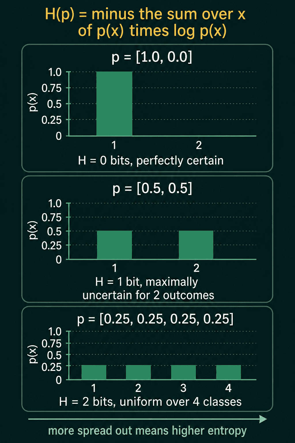
In general, $k$ equally likely outcomes give $H = \log k$, and no distribution over $k$ outcomes has higher entropy. Any other distribution is more concentrated, so its entropy comes out lower.
Entropy as the length of a code
Entropy also counts bits in the literal sense. Suppose you need to send which of 16 equally likely outcomes happened. A fixed code of 4 bits per message labels all 16 outcomes, since $2^4 = 16$, and 4 bits is exactly the entropy $\log_2 16$.
Now make the 16 outcomes lopsided. The first has probability 1/2 and the second 1/4, each next one is half the one before, and the last two have $1/2^{15}$ each. Give the frequent outcomes short codes (0, then 10, then 110) and the rare ones long codes. The average message length drops to about 2.00 bits, which is the entropy of this distribution.
That is Shannon's noiseless coding theorem: entropy is the minimum average number of bits needed to send a variable's value, and no code beats it on average. Codes can only get close to it in general, and they reach it exactly here because every probability is a power of 1/2.
Bits and nats
The base of the log sets the unit and nothing else. Base 2 gives bits. The natural log, $\ln$ (base $e \approx 2.718$), gives nats. One nat is $1/\ln 2 \approx 1.44$ bits, so the fair coin has entropy 1 bit, or $\ln 2 \approx 0.693$ nats.
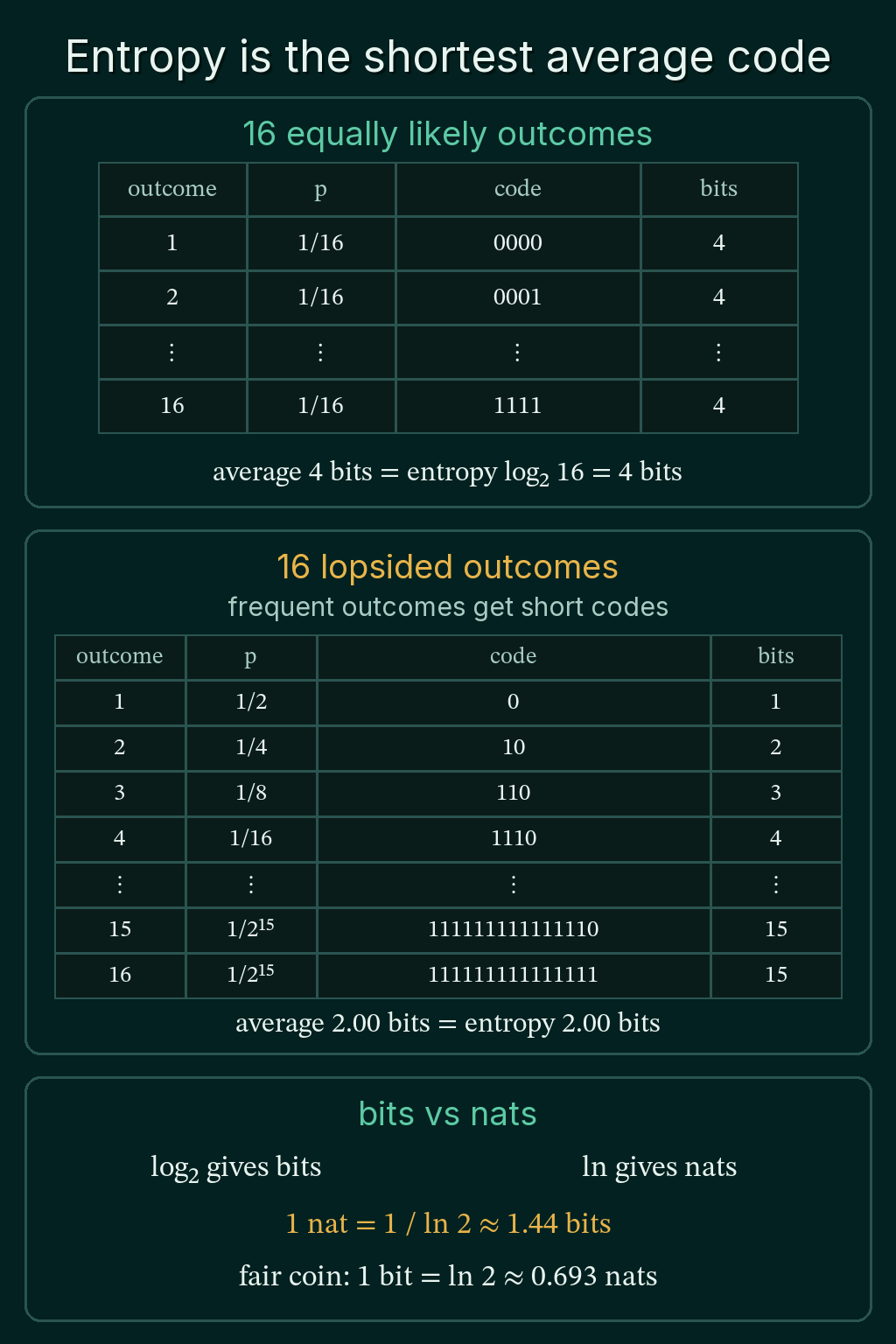
torch.log and np.log are natural logs, so entropies computed in ML code are in nats unless someone divides by $\ln 2$. A value that looks off by a factor of about 1.44 is usually this.
Entropy in PyTorch
The function below drops the zero probabilities first, which applies the $0 \log 0 = 0$ convention. Then it sums $p \log(1/p)$, which equals $-p \log p$:
1import torch
2
3def entropy(p):
4    p = p[p > 0]                          # 0 log 0 counts as 0
5    return (p * torch.log(1 / p)).sum()   # natural log, so the result is in nats
6
7for p in ([0.5, 0.5], [0.99, 0.01], [0.25, 0.25, 0.25, 0.25], [1.0, 0.0]):
8    h = entropy(torch.tensor(p))
9    print(f"{str(p):26} {h:.4f} nats   {h / torch.log(torch.tensor(2.0)):.4f} bits")
10# [0.5, 0.5]                 0.6931 nats   1.0000 bits
11# [0.99, 0.01]               0.0560 nats   0.0808 bits
12# [0.25, 0.25, 0.25, 0.25]   1.3863 nats   2.0000 bits
13# [1.0, 0.0]                 0.0000 nats   0.0000 bits
PyTorch also has it built in for a distribution over categories. The weather forecast from earlier comes out at 0.80 nats, which is about 1.16 bits:
1import torch
2
3p = torch.tensor([0.7, 0.2, 0.1])
4print(torch.distributions.Categorical(probs=p).entropy())   # in nats
5# tensor(0.8018)
If an entropy comes out as nan, check for a zero probability first.
Differential entropy: entropy for continuous variables
Everything so far had a list of outcomes, each with its own probability. A height, a temperature or a predicted price can take infinitely many values, so no single value has a meaningful probability on its own. A continuous variable is described by a density $p(x)$ instead, and the probability of landing in a range is the area under the density over that range.
A density is not a probability and can be larger than 1. Take a value that lands somewhere between 0 and 0.5, with every point in that range equally likely. This is a uniform distribution. Its total area has to be 1 and the range is only 0.5 wide, so the density is $1 / 0.5 = 2$ across the whole range.
Entropy carries over to densities by turning the sum into an integral. This is called differential entropy, written with a lowercase $h$:
$$h(p) = -\int p(x) \log p(x)\, dx$$
The uniform density is $p(x) = 2$ on a range of width 0.5, so the integral is $-0.5 \cdot 2 \ln 2 = -\ln 2 = \ln 0.5 \approx -0.69$ nats. The answer is negative. Discrete entropy can never be negative, because every probability is at most 1, so every $\log p(x)$ is zero or negative and the minus sign makes each term non-negative. A density above 1 has a positive log, and that term flips sign.
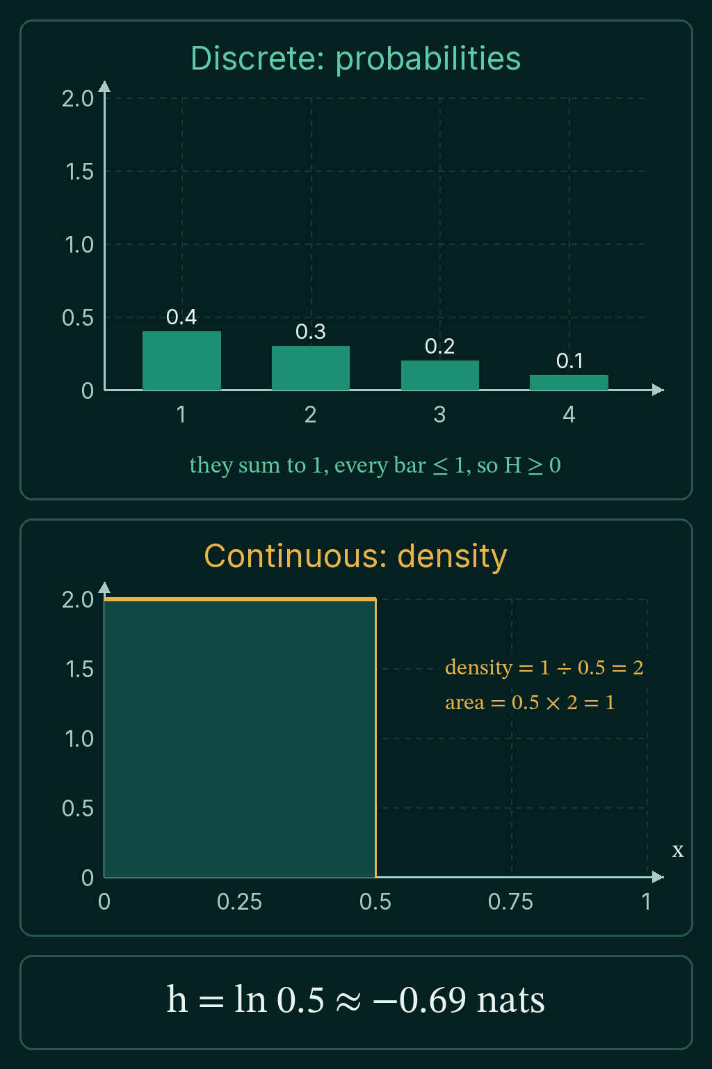
A negative differential entropy does not mean something went wrong. It means the variable is pinned into a range narrower than one unit of $x$.
The Gaussian: the width decides the sign
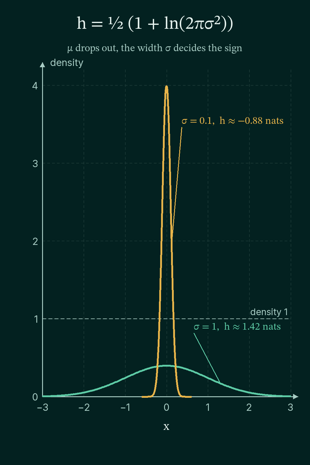
The Gaussian (or normal) distribution is the bell curve. Its mean $\mu$ slides the bell left or right, and its standard deviation $\sigma$ sets the width. Putting its density into the integral and working through the calculus gives
$$h = \frac{1}{2}\big(1 + \ln(2\pi\sigma^2)\big)$$
The mean $\mu$ is gone, so moving the bell left or right does not change its entropy. With $\sigma = 1$ the entropy is about 1.42 nats, and with $\sigma = 0.1$ it is about $-0.88$ nats:
1import torch
2
3for sigma in (1.0, 0.1):
4    h = torch.distributions.Normal(0.0, sigma).entropy()
5    print(f"sigma {sigma}: h = {h:.3f} nats")
6print(torch.distributions.Uniform(0.0, 0.5).entropy())
7# sigma 1.0: h = 1.419 nats
8# sigma 0.1: h = -0.884 nats
9# tensor(-0.6931)
Differential entropy also depends on the units of $x$. Measure the same heights in centimeters instead of meters and $\sigma$ grows 100 times, which adds $\ln 100 \approx 4.6$ nats to $h$ even though nothing about the uncertainty changed. A single differential entropy value says little on its own. Comparing two distributions of the same variable is where it stays useful, which is what cross-entropy and KL divergence do.
The maximum entropy principle
So far entropy was measured on a distribution that was already known. The maximum entropy principle uses it the other way: to choose a distribution when only a few facts are known.
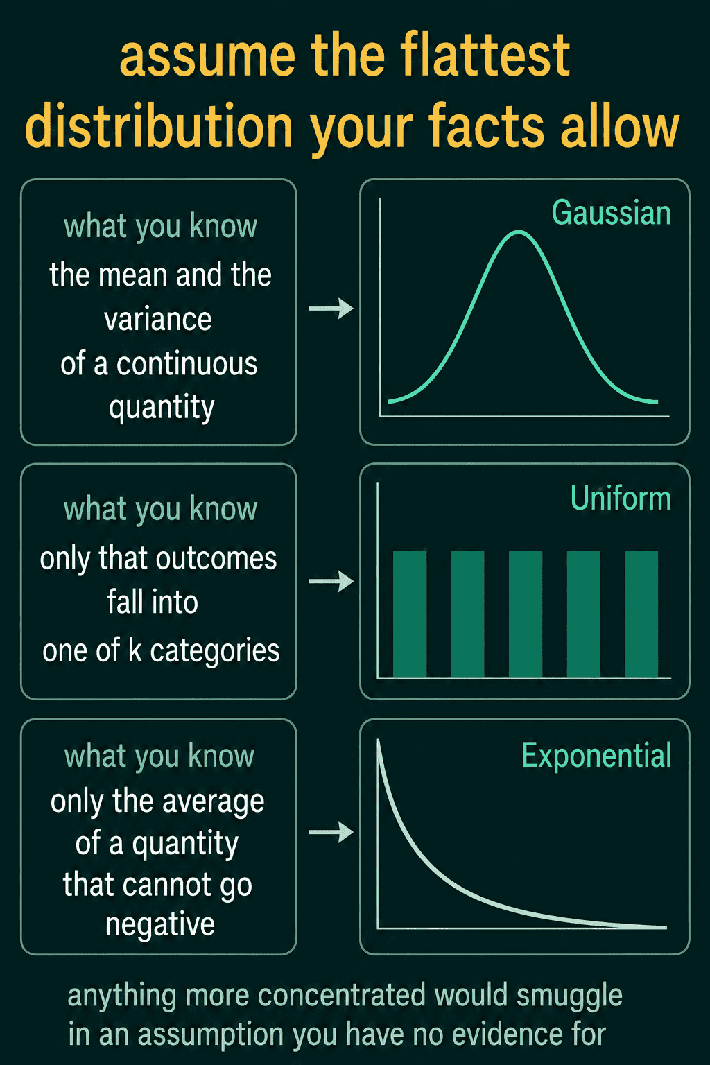
Say you know the mean and the variance of a quantity, and nothing else. Infinitely many distributions share that mean and variance. The principle says to pick the one with the highest entropy among them, because any more concentrated choice assumes something the facts do not support. Different facts give different answers:
- Only that the outcome is one of $k$ categories: the uniform distribution, $1/k$ each.
- The mean and the variance of a continuous quantity: the Gaussian. This is one reason Gaussian noise is a common default in ML models, as the least committal choice when a mean and a variance are all that is known.
- Only the mean of a quantity that cannot be negative, like a wait time: the exponential distribution, which starts highest at zero and decays from there.
Written as an optimization problem, the principle is
$$\max_p \; H(p) \quad \text{subject to} \quad \sum_x p(x) = 1, \quad p(x) \geq 0$$
plus a constraint for each extra fact: $E[x] = \mu$ and $E[(x - \mu)^2] = \sigma^2$ for the Gaussian, where $E$ is the expected value (the probability-weighted average), or $E[x] = \mu$ with $x \geq 0$ for the exponential.
The discrete case can be checked by hand. With four categories and nothing else known, the uniform $p = [0.25, 0.25, 0.25, 0.25]$ has entropy $\log_2 4 = 2$ bits. Move one probability up to 0.4 and the other three down to 0.2 each, and the entropy drops to
$$-(0.4 \log_2 0.4 + 3 \cdot 0.2 \log_2 0.2) \approx 1.92 \text{ bits}$$
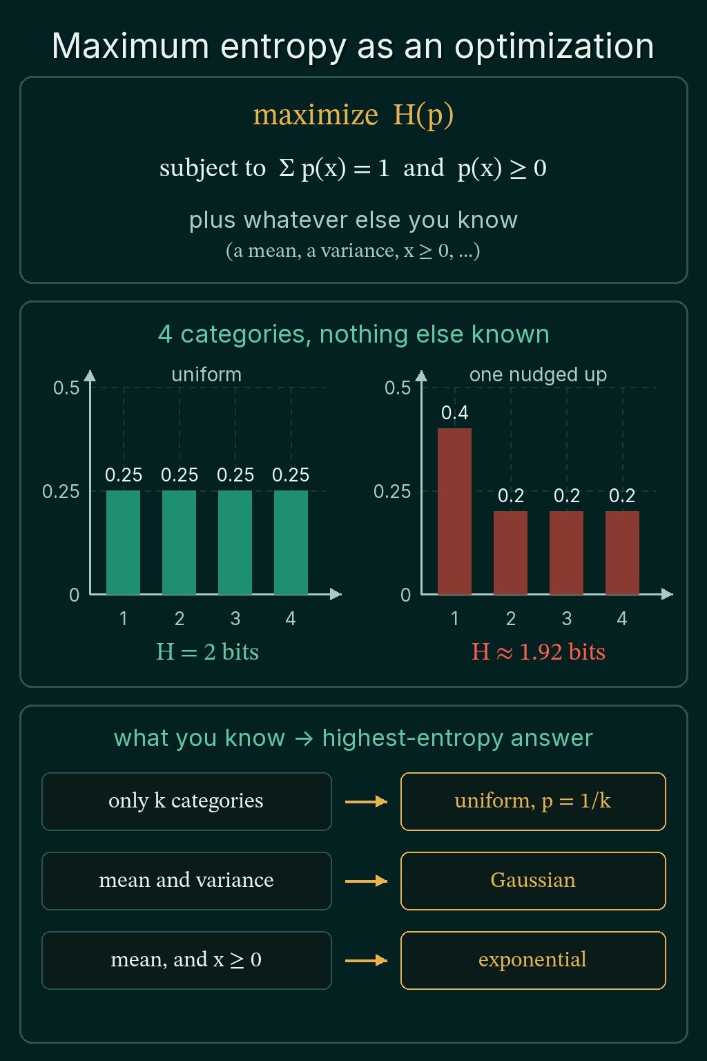
The Gaussian and exponential answers come out of the same optimization with the extra constraints attached, using Lagrange multipliers. The uniform, Gaussian and exponential are the same rule applied to different facts.
When entropy is useful, and common mistakes
Use entropy to measure how spread out a single distribution is: how confident a classifier's predicted probabilities are, how mixed the labels at a decision tree node are, or how many bits a value needs on average. To compare two distributions, cross-entropy and KL divergence are the tools.
- Mixing bits and nats. A result computed with
torch.logis in nats. Divide by $\ln 2$ before comparing it with a number in bits. - Getting
nanfrom a zero probability.torch.log(0.0)is-inf, and0 * -infisnan, so a raw-(p * torch.log(p)).sum()on[0.5, 0.5, 0.0]returnsnaninstead of 0.693. Drop the zeros first, as in the function above. - Reading a differential entropy value as an absolute amount of uncertainty. It can be negative and it shifts when the units of $x$ change.
Related concepts
Entropy, cross-entropy and KL divergence builds from entropy to the loss most classifiers train with. Mutual information uses entropy to measure how much one variable says about another. The Gaussian distribution covers the bell curve whose entropy depends only on its width.
QuiddityML teaches self-information, entropy, differential entropy and the maximum entropy principle as four concepts in the Math track's information theory unit. The exercises on entropy include writing entropy(p) from scratch and spotting the bug in an entropy function.