By Sagi Shaier · 14 October 2026 · 5 min read

Random variables and probability distributions explained: PMF vs PDF

How a die roll and a classifier's output are both described by a distribution, the two rules every distribution follows, and why a density can be larger than 1 while a probability cannot, with PyTorch code.

A random variable is a quantity whose value is uncertain until you observe it, and a probability distribution says how likely each of its values is. ML uses them wherever a model deals with uncertainty, such as the class label of an image or the next token in a sentence. The tool that describes the distribution depends on whether the values are separate categories or numbers on a continuous scale.

Random variables

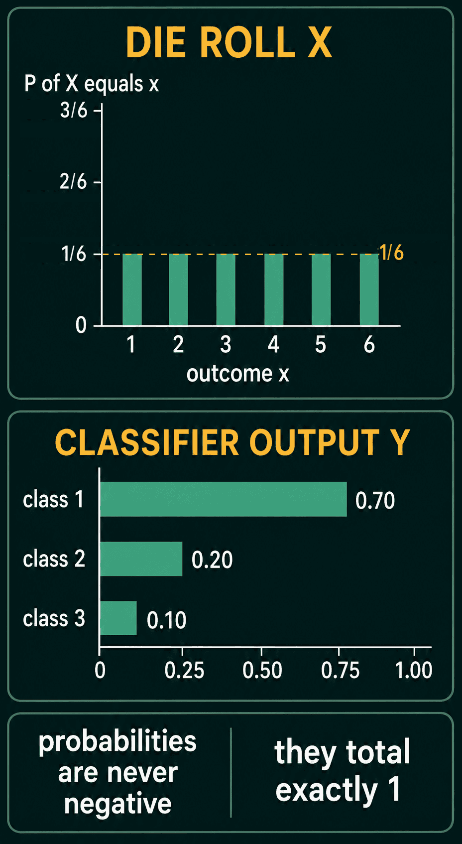
A random variable is usually written as a capital letter. For a six-sided die, $X$ is the result of the roll. Before the roll, $X$ could be any whole number from $1$ to $6$, and its distribution gives each value the same probability:

$$P(X=1) = P(X=2) = \dots = P(X=6) = \frac{1}{6}$$

$P(X = 4)$ reads "the probability that $X$ equals 4".

Three more words come with every distribution. An outcome is one thing that can happen, such as rolling a 4. The sample space is the set of all outcomes, here $\{1, 2, 3, 4, 5, 6\}$. An event is any set of outcomes you can ask the probability of. "The roll is at least 5" is the event $\{5, 6\}$, with probability $2/6 = 1/3$. A random variable taking one value, such as $X = 4$, is also an event.

Distributions in ML

A classifier's output is a distribution too. For an image classifier with three classes, the random variable $Y$ is the class label. A softmax layer turns the model's raw scores into probabilities by exponentiating each score and dividing by the total. An output of $[0.70, 0.20, 0.10]$ says the model gives class 1 a probability of 70%, class 2 a probability of 20% and class 3 a probability of 10%.

Every distribution follows two rules:

No probability is negative.
The probabilities of all possible outcomes add up to 1.

The second rule is what separates a distribution from a list of scores. Raw scores can be any numbers, while probabilities have to account for every outcome between them. An output of $[0.6, 0.6]$ over two labels breaks the rule, since it adds up to $1.2$.

A bar chart of a fair die roll X with every outcome from 1 to 6 at probability 1 over 6, above a bar chart of a classifier output Y with class 1 at 0.70, class 2 at 0.20 and class 3 at 0.10, and the two rules: probabilities are never negative and they total exactly 1

The probability mass function (PMF)

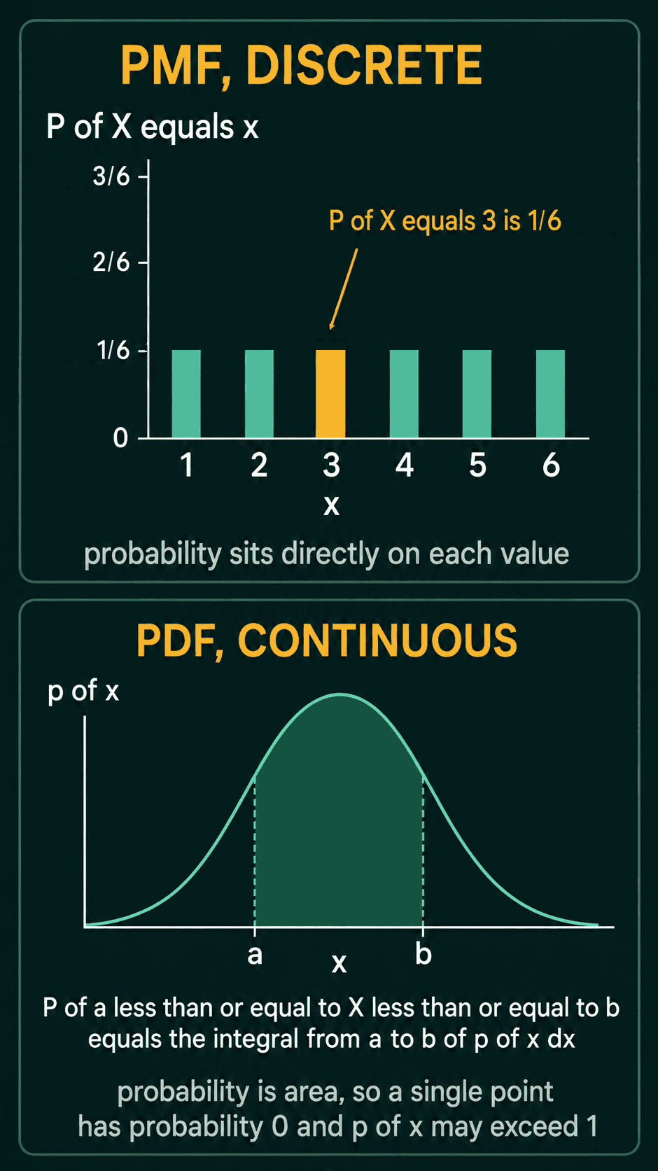
When the values are separate, such as die faces or class labels, the random variable is discrete. A probability mass function, or PMF, gives each value its probability directly:

$$P(X = x)$$

Here the lowercase $x$ is one particular value and the capital $X$ is the random variable. A valid PMF follows the two rules from above, written as formulas:

$$P(X = x) \geq 0$$

$$\sum_x P(X = x) = 1$$

The $\sum_x$ means add over every possible value. For the die, $P(X = 3) = 1/6$, and the six values of $1/6$ add up to 1. Each entry of a PMF is a real probability, so no entry can be larger than 1.

The probability density function (PDF)

Height, temperature and regression errors take values on a continuous scale, so these random variables are continuous. Between any two heights there are infinitely many others. So the probability of one exact value is 0, for example a height of exactly 172.000 cm with every further digit zero. A probability density function (PDF), written $p(x)$, handles this by giving probability to intervals. The probability that $X$ lands between $a$ and $b$ is the area under $p(x)$ from $a$ to $b$:

$$P(a \le X \le b) = \int_a^b p(x)\,dx$$

The integral sign $\int_a^b$ stands for the area under the curve between $a$ and $b$. The two rules become

$$p(x) \geq 0$$

$$\int_{-\infty}^{\infty} p(x)\,dx = 1$$

so the density is never negative and the total area under the curve is 1.

A PMF for a fair die with probability sitting directly on each value and P of X equals 3 highlighted at 1 over 6, above a bell-shaped PDF where the probability of landing between a and b is the shaded area under the curve, so a single point has probability 0 and p of x may exceed 1

Why a density can be larger than 1

A value of $p(x)$ is a density, not a probability, so it can be larger than 1. Take a random variable that is equally likely to land anywhere between 0 and 0.5. The total area has to be 1 on an interval of width 0.5, so the density has to be $p(x) = 2$ on that interval. The probability of landing between 0.1 and 0.3 is the area of a rectangle with width 0.2 and height 2:

$$P(0.1 \le X \le 0.3) = 0.2 \cdot 2 = 0.4$$

The density is 2 everywhere on the interval, and every probability computed from it still lands between 0 and 1.

PMFs and PDFs in PyTorch

torch.softmax turns raw scores into a PMF over classes. Rolling a simulated die many times gives frequencies close to the die's PMF:

1import torch
2 
3logits = torch.tensor([2.0, 0.5, -0.3])
4probs = torch.softmax(logits, dim=0)
5print(probs)          # one probability per class
6print(probs.sum())    # adds to 1
7 
8rolls = torch.randint(1, 7, (60_000,), generator=torch.Generator().manual_seed(0))
9counts = torch.bincount(rolls, minlength=7)[1:]
10print(counts / len(rolls))    # each close to 1/6 = 0.1667
11# tensor([0.7556, 0.1686, 0.0758])
12# tensor(1.)
13# tensor([0.1678, 0.1658, 0.1670, 0.1678, 0.1651, 0.1665])

For a PDF, Normal(loc=0.0, scale=0.1) is a bell-shaped density centred at 0 with its width set by scale. A narrow bell has to be tall to keep its total area at 1. cdf(b) gives the probability of landing at or below b, so the difference of two cdf values is the probability of an interval:

1import torch
2from torch.distributions import Normal
3 
4narrow = Normal(loc=0.0, scale=0.1)
5print(narrow.log_prob(torch.tensor(0.0)).exp())    # density at 0, above 1
6 
7# probability of an interval = area under the density
8a, b = torch.tensor(-0.1), torch.tensor(0.1)
9print(narrow.cdf(b) - narrow.cdf(a))
10 
11# the same area by adding up density times a small width
12xs = torch.linspace(-0.1, 0.1, 2001)
13width = xs[1] - xs[0]
14print((narrow.log_prob(xs).exp() * width).sum())
15# tensor(3.9894)
16# tensor(0.6827)
17# tensor(0.6829)

The density at 0 is about 3.99. The probability of landing between $-0.1$ and $0.1$ is 0.6827, and adding density times a small width over the same range gives 0.6829, close to the exact area. If a number you expected to be a probability comes out above 1, check whether the code returned a density instead.

When to use which, and common mistakes

Use a PMF for anything that comes in separate values: class labels, tokens, or counts such as the number of users who click a button today. Use a PDF for values on a continuous scale: noise models, regression errors and latent variables, which are quantities a model reasons about but never observes directly.

Reading a density as a probability. A density of 3.99 is not a 399% chance. Probabilities come from areas under the density.
Asking for the probability of one exact continuous value. It is 0, so ask about an interval.
Outputs that do not add up to 1. $[0.6, 0.6]$ is not a distribution, which is why classifiers pass their raw scores through softmax.

Joint and conditional probability describe two random variables at once, such as an image and its label. The cumulative distribution function (CDF) gives the probability of landing at or below a value, and the difference of two CDF values is the interval probability computed above. Common distributions, such as the Bernoulli for one yes-or-no outcome and the Gaussian for bell-shaped continuous values, are specific PMFs and PDFs with names.

QuiddityML teaches random variables and the PMF vs PDF difference as two concepts in the Math track. The exercises on them include spotting what is wrong with a [0.6, 0.6] output and matching code that adds up density times bin width to the integral it approximates.