By Sagi Shaier · 20 October 2026 · 5 min read

Bootstrap resampling explained

How to get a standard error and a 95% interval for a median, an accuracy or any other statistic without deriving a formula, with the PyTorch code and the mistakes to avoid.

Bootstrap resampling estimates how much a statistic would change across datasets by building many new datasets out of the one you have and recomputing the statistic on each. It gives error bars for statistics that have no simple formula for their uncertainty, like a median or a correlation.

What problem does the bootstrap solve?

A statistic computed from data changes from one dataset to the next. The standard error is the typical size of that change, measured as the standard deviation of the statistic across datasets. For a sample mean there is a formula, $s/\sqrt{n}$, where $s$ is the standard deviation of the data and $n$ is the number of rows. With $s = 10$ and $n = 25$, the mean has a standard error of $10/5 = 2$.

Now try writing one for a median, a correlation, or a coefficient fitted by a model. For most statistics the formula either does not exist in closed form or takes a page of assumptions to reach. The bootstrap skips the derivation: instead of working out how much a statistic would vary across datasets, it makes more datasets and looks.

How a bootstrap sample is built

Start with a dataset of $n$ rows. A bootstrap sample (or resample) is another dataset of $n$ rows drawn from the original with replacement. That means each drawn row goes back before the next draw and can be drawn again. Some original rows appear more than once, and some do not appear at all.

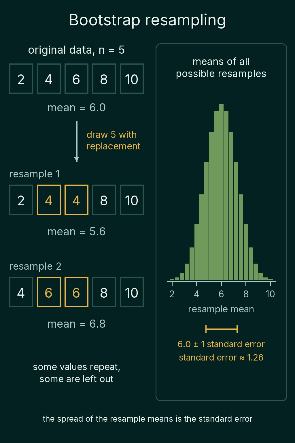
For example, take the five values $2, 4, 6, 8, 10$ with mean 6.0. One resample is $2, 4, 4, 8, 10$, where 4 appears twice and 6 is left out. Its mean is 5.6. Another resample is $4, 6, 6, 8, 10$ with mean 6.8.

In PyTorch, idx = torch.randint(0, n, (n,)) draws n random row positions from 0 to n - 1 with repeats allowed, and data[idx] builds the resample.

From resamples to a standard error

Compute the statistic on each resample, repeat many times, and take the standard deviation of the results. That standard deviation is the bootstrap standard error. The number of resamples is usually written $B$.

Five values allow $5^5 = 3{,}125$ different ordered resamples. The means of all of them form the histogram below, centered on 6.0 with a standard deviation of about 1.26, which is the bootstrap standard error of the mean for this data:

The data 2 to 10 with mean 6.0 and two resamples with their repeated values in amber, next to a histogram of the means of all possible resamples centered on 6 with a bar marking one standard error of about 1.26 on each side.

The mean is a useful test case because the formula exists. The code below draws 40 skewed values that stand for response times in milliseconds. It compares the bootstrap standard error from 10,000 resamples with $s/\sqrt{n}$:

1import torch
2 
3torch.manual_seed(0)
4data = torch.distributions.Exponential(1 / 200.0).sample((40,))   # 40 response times in ms
5n, B = len(data), 10_000
6 
7idx = torch.randint(0, n, (B, n))         # B resamples, each n row positions drawn with repeats
8means = data[idx].mean(dim=1)              # one mean per resample
9 
10print(f"mean of the data      {data.mean():.1f}")
11print(f"bootstrap SE          {means.std():.1f}")
12print(f"formula s / sqrt(n)   {data.std() / n**0.5:.1f}")
13# mean of the data      227.2
14# bootstrap SE          32.8
15# formula s / sqrt(n)   33.1

The two agree to within 0.3 ms. The same code works for any statistic by replacing .mean(dim=1) with something else.

From resamples to an interval

A standard error is a single number, and an interval is usually what gets reported. Sort the $B$ bootstrap estimates and read off the 2.5th and 97.5th percentiles, the values below which 2.5% and 97.5% of the estimates fall. That pair is a 95% percentile interval.

A $\bar{x} \pm 1.96\,\mathrm{SE}$ interval is symmetric around the estimate by construction. A percentile interval comes from wherever the bootstrap estimates actually landed, so it can be lopsided when the statistic's distribution is. The code below does this for the median of the same 40 response times:

1import torch
2 
3torch.manual_seed(0)
4data = torch.distributions.Exponential(1 / 200.0).sample((40,))
5n, B = len(data), 10_000
6idx = torch.randint(0, n, (B, n))
7 
8medians = data[idx].median(dim=1).values
9lo, hi = torch.quantile(medians, torch.tensor([0.025, 0.975]))
10print(f"median {data.median():.1f}   95% interval [{lo:.1f}, {hi:.1f}]")
11# median 149.7   95% interval [103.0, 221.6]

The interval reaches 46.7 ms below the median and 71.9 ms above it, because response times have a long tail of slow values on the right.

Why it works

The bootstrap treats the original dataset as a stand-in for the full population it came from. Drawing resamples from it imitates drawing new datasets from the population, so the spread of the statistic across resamples approximates its spread across real datasets. The picture is rough when the dataset is small, since a handful of rows is a poor stand-in for a population.

The bootstrap in machine learning

A model's accuracy on a test set is a statistic too, and resampling the test examples gives it an interval. Here a model gets 172 of 200 test examples right:

1import torch
2 
3torch.manual_seed(0)
4correct = torch.zeros(200)
5correct[:172] = 1                          # 172 of 200 test examples right: 86% accuracy
6idx = torch.randint(0, 200, (10_000, 200))
7acc = correct[idx].mean(dim=1)
8lo, hi = torch.quantile(acc, torch.tensor([0.025, 0.975]))
9print(f"accuracy {correct.mean():.3f}   95% interval [{lo:.3f}, {hi:.3f}]")
10# accuracy 0.860   95% interval [0.810, 0.905]

The 86% accuracy comes with an interval from 81.0% to 90.5%, so a second model scoring 88% on the same 200 examples has not clearly beaten it.

Resampling also shows up inside models. Bagging trains several models on different bootstrap samples of the training data and averages their predictions, and a random forest does this with decision trees. Each tree sees a slightly different dataset and learns slightly different splits, and averaging them reduces the variance of the prediction.

When to use it, and common mistakes

The bootstrap fits when a statistic has no convenient standard error formula, or when its distribution may be lopsided and a symmetric interval would misrepresent it.

Sampling without replacement. data[torch.randperm(n)] only shuffles the rows, so every resample has the same mean and the standard error comes out as 0.
Resamples of a different size. Each resample needs $n$ rows. Smaller resamples spread more and overstate the uncertainty.
Too few resamples. The 2.5th and 97.5th percentiles of 100 estimates rest on two or three values each. A few thousand resamples is a common choice.
Expecting it to rescue a tiny dataset. Resampling cannot add information that the original rows do not have.

Standard error and confidence intervals covers the formula-based intervals the bootstrap is compared with here. CDF, percentiles and quantiles explains the percentiles that a percentile interval reads off. Bias and variance of an estimator covers the spread across datasets that the bootstrap approximates. Monte Carlo methods uses the same idea of estimating a quantity by averaging over random draws.

QuiddityML teaches bootstrap resampling in the Math track's probability unit, and the exercises on it include filling in the torch.randint line that draws a resample and writing bootstrap_se from scratch.