By Sagi Shaier · 20 October 2026 · 5 min read
The reparameterization trick explained
How to build a Gaussian sample from a mean, a Cholesky factor and standard normal noise, why that lets gradients reach the mean, and how PyTorch's rsample does it for you.
The reparameterization trick turns a random sample, which cannot be differentiated, into a formula that can. Training needs the derivative of the loss with respect to every learned number, and drawing a sample from a distribution has no derivative with respect to its mean or its spread. The trick first draws plain random noise and then computes the sample from it as the mean plus the spread times the noise. That formula can be differentiated with respect to the mean and the spread, and the noise is the only random part left. Models that sample in the middle of their computation need this, and a well-known example is the variational autoencoder (a model that learns to generate new data such as images).
What problem does it solve?
Training a model means computing the gradient of the loss with respect to every parameter and moving each parameter a little against it. Backpropagation gets those gradients by following the chain of operations from the loss back to the parameters.
Suppose a model computes a mean $\mu$ and then draws a sample $z$ from a normal distribution with that mean. If $\mu$ moves from 3 to 3.1, nothing says how $z$ should move, because a fresh draw can land anywhere. So the gradient of the loss stops at $z$ and never reaches $\mu$ or the parameters that produced it.
Sampling a Gaussian through a transform
Start in one dimension. Let $\epsilon$ be a sample from a standard normal, which has mean 0 and standard deviation 1. Then
$$z = \mu + \sigma \epsilon$$
is a sample from a normal distribution with mean $\mu$ and standard deviation $\sigma$. Multiplying by $\sigma$ stretches the spread, and adding $\mu$ moves the center. For example, take $\mu = 3$ and $\sigma = 2$. A noise draw of $\epsilon = 0.5$ gives $z = 4$, and $\epsilon = -1$ gives $z = 1$.
Now $z$ is an ordinary formula. Its derivative with respect to $\mu$ is 1, and its derivative with respect to $\sigma$ is $\epsilon$. The randomness lives entirely in $\epsilon$, which does not depend on any parameter.
The multivariate version
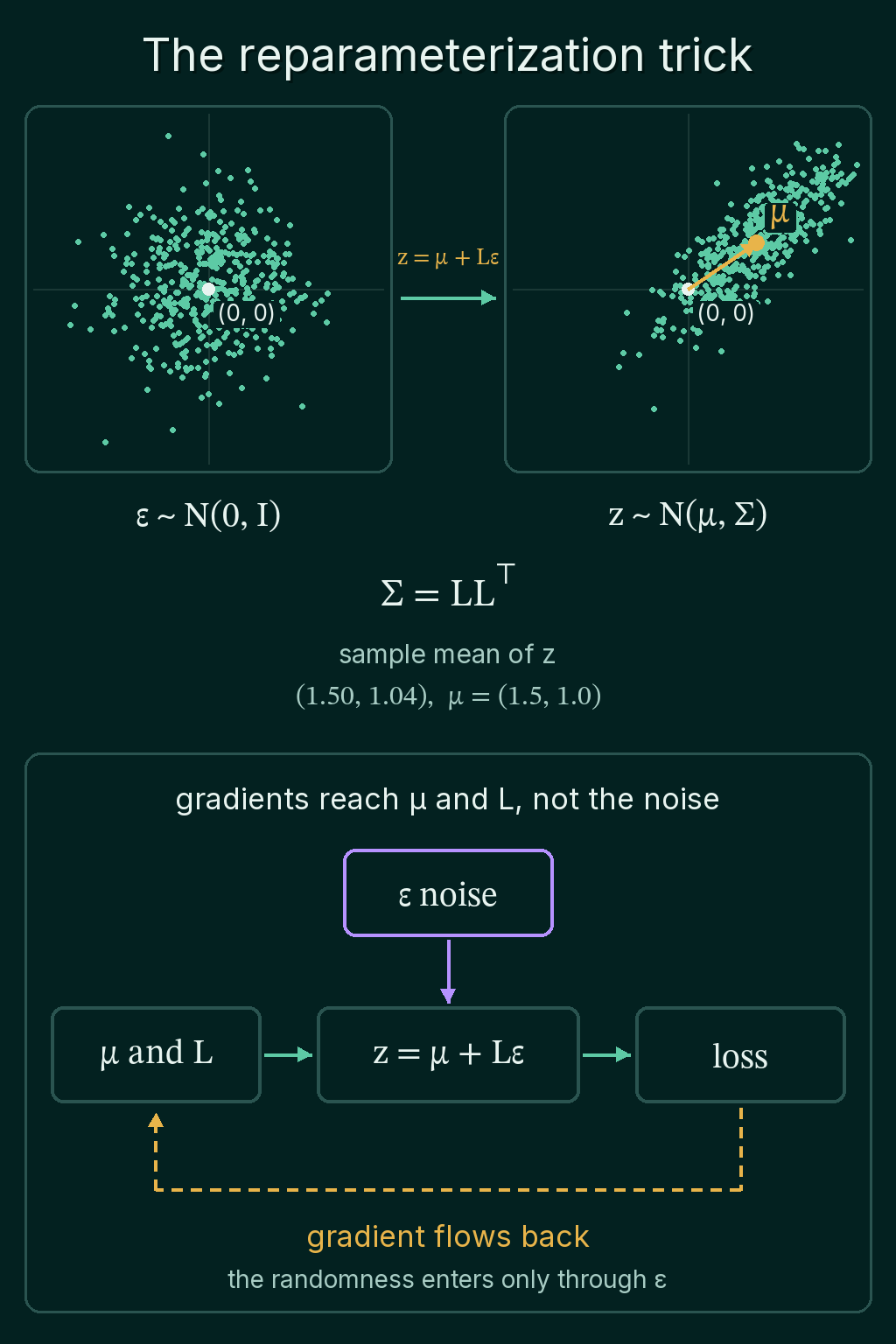
In more than one dimension, the spread is a covariance matrix $\Sigma$, whose diagonal holds each coordinate's variance and whose off-diagonal entries say how pairs of coordinates move together. The noise $\boldsymbol{\epsilon}$ is now a vector of independent standard normals, with mean 0 and identity covariance $I$. The sample is
$$\mathbf{z} = \boldsymbol{\mu} + L\boldsymbol{\epsilon}$$
$$\Sigma = LL^\top$$
Here $L$ is any matrix whose product with its own transpose gives $\Sigma$, a kind of square root of the covariance matrix. The usual choice is the lower-triangular one, called the Cholesky factor, which torch.linalg.cholesky(Sigma) computes.
For example, take the mean $\boldsymbol{\mu} = (1.5, 1.0)$ and
$$\Sigma = \begin{pmatrix} 1 & 0.75 \\ 0.75 & 0.9 \end{pmatrix}$$
The Cholesky factor is
$$L = \begin{pmatrix} 1 & 0 \\ 0.75 & 0.581 \end{pmatrix}$$
You can check it by hand: the bottom-right entry of $LL^\top$ is $0.75^2 + 0.581^2 \approx 0.5625 + 0.3375 = 0.9$. A noise vector $\boldsymbol{\epsilon} = (1, 2)$ gives $L\boldsymbol{\epsilon} = (1,\ 0.75 + 1.162) = (1, 1.912)$, so $\mathbf{z} = (2.5, 2.912)$.
The covariance comes out right because a matrix $L$ turns a covariance $\Sigma_0$ into $L\Sigma_0L^\top$. With $\Sigma_0 = I$ that gives $LIL^\top = LL^\top = \Sigma$. Adding $\boldsymbol{\mu}$ then moves the center without changing the spread. The code below draws 100,000 samples this way and checks both:
1import torch
2
3mu = torch.tensor([1.5, 1.0])
4Sigma = torch.tensor([[1.0, 0.75],
5                      [0.75, 0.9]])
6L = torch.linalg.cholesky(Sigma)         # lower-triangular, L @ L.T == Sigma
7print(L)
8
9torch.manual_seed(0)
10eps = torch.randn(100_000, 2)            # standard normal: mean 0, covariance I
11z = mu + eps @ L.T                       # z = mu + L eps, one row per sample
12print(z.mean(dim=0))
13print(torch.cov(z.T))
14# tensor([[1.0000, 0.0000],
15#         [0.7500, 0.5809]])
16# tensor([1.4976, 0.9954])
17# tensor([[0.9957, 0.7493],
18#         [0.7493, 0.9030]])
The samples are stored one per row, so eps @ L.T applies $L$ to every row at once. The sample mean is within 0.005 of $\boldsymbol{\mu}$, and the sample covariance is within 0.005 of $\Sigma$ in every entry.
Why gradients now reach the mean
Since $\mathbf{z} = \boldsymbol{\mu} + L\boldsymbol{\epsilon}$, the noise is an input drawn before the formula runs. Everything between $\boldsymbol{\mu}$ and the loss is ordinary arithmetic, so backpropagation can carry the gradient from the loss to $\boldsymbol{\mu}$ and $L$. Writing a draw this way is the reparameterization trick:
The code below learns a mean and a spread by gradient descent through the sampling step. The loss is the average squared distance of the samples from 3. The spread is stored as $\log \sigma$ and exponentiated, which keeps $\sigma$ positive whatever value the optimizer gives $\log \sigma$:
1import torch
2
3torch.manual_seed(0)
4mu = torch.tensor(0.0, requires_grad=True)
5log_sigma = torch.tensor(0.0, requires_grad=True)
6opt = torch.optim.SGD([mu, log_sigma], lr=0.05)
7
8for step in range(300):
9    eps = torch.randn(256)                     # the randomness, drawn on its own
10    z = mu + log_sigma.exp() * eps             # differentiable in mu and log_sigma
11    loss = ((z - 3.0) ** 2).mean()             # want samples close to 3
12    opt.zero_grad()
13    loss.backward()
14    opt.step()
15
16print(f"mu {mu.item():.3f}  sigma {log_sigma.exp().item():.3f}")
17# mu 2.997  sigma 0.128
The mean moved from 0 to 2.997, and the spread shrank from 1 to 0.128, because any spread around 3 adds to this loss. Both parameters received gradients through $z$.
rsample in PyTorch
PyTorch distributions have two sampling methods. .sample() returns a value with no gradient path, and .rsample() builds the sample with the reparameterization trick:
1import torch
2from torch.distributions import Normal
3
4mu = torch.tensor(0.0, requires_grad=True)
5dist = Normal(mu, 1.0)
6
7z = dist.sample()
8print(z.requires_grad)                   # no path back to mu
9
10z = dist.rsample()                       # mu + 1.0 * eps under the hood
11print(z.requires_grad)
12# False
13# True
torch.distributions.MultivariateNormal(mu, Sigma).rsample() does the multivariate version, computing the Cholesky factor internally.
When to use it, and common mistakes
Use it when a loss depends on a sample and the distribution's parameters are being learned. Variational autoencoders are built on it. When samples are only being generated, with no gradient needed, .sample() is fine.
- Calling
.sample()inside the training path. The parameters of the distribution get no gradient from the loss, so they stay where they started. - Multiplying by $\Sigma$ instead of $L$. $\boldsymbol{\mu} + \Sigma\boldsymbol{\epsilon}$ has covariance $\Sigma\Sigma^\top$, which is the wrong spread.
- Writing
eps @ Lfor a batch stored as rows. The batched form of $L\boldsymbol{\epsilon}$ iseps @ L.T, andeps @ Lgives covariance $L^\top L$ instead of $LL^\top$. - Learning $\sigma$ directly. Gradient steps can push it below zero. Learning $\log \sigma$ and exponentiating avoids that.
Related concepts
The multivariate Gaussian post explains covariance matrices and the shapes they produce. Positive definite matrices, Cholesky and QR covers where the Cholesky factor comes from. Backpropagation is the algorithm that carries the gradient through $\mathbf{z} = \boldsymbol{\mu} + L\boldsymbol{\epsilon}$. Monte Carlo methods explains why averaging the loss over many samples estimates its expected value.
QuiddityML teaches the reparameterization trick in the Math track's probability unit, and the exercises on it include picking the line of code that implements $\mathbf{z} = \boldsymbol{\mu} + L\boldsymbol{\epsilon}$ and writing reparameterize from scratch with torch.linalg.cholesky.