By Sagi Shaier · 20 October 2026 · 6 min read
Markov chain Monte Carlo (MCMC) explained
How the Metropolis-Hastings rule decides each step, why the unknown normalizing constant never has to be computed, and how many independent draws a correlated chain is worth, with a working sampler in PyTorch.
Markov chain Monte Carlo (MCMC) draws samples from a distribution by taking a random walk whose visited points end up spread out like that distribution. It is a common way to sample from a Bayesian posterior, where the density can be written down up to an unknown constant but cannot be sampled from directly.
What problem does MCMC solve?
Monte Carlo estimation approximates an expected value by averaging over samples from a distribution, called the target $p(x)$. When the target cannot be sampled directly, importance sampling and rejection sampling draw from an easier distribution $q(x)$ instead. That distribution is called the proposal, and both methods correct for the difference afterwards. Both need a single proposal that covers the target across the whole space at once.
That gets hard in many dimensions. A rejection sampler whose proposal is a normal distribution only 1.1 times wider than a 50-dimensional normal target keeps under 1% of its draws, as the PyTorch run in Monte Carlo methods explained shows. MCMC avoids the problem by giving up on independent draws.
The random walk
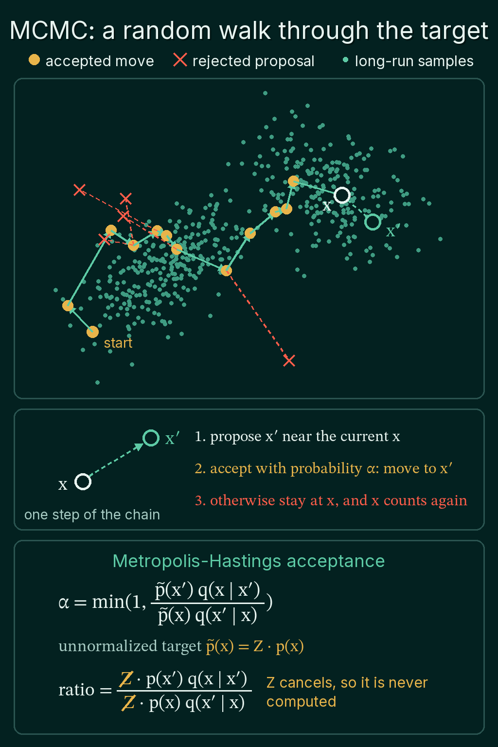
Instead of drawing every sample from scratch, MCMC builds a chain: a sequence of states $x_1, x_2, x_3, \dots$ in which each new state is proposed near the current one and then accepted or rejected. A random process whose next step depends only on where it is now is called a Markov chain, which is where the name comes from.
The rule for accepting or rejecting is built so that the chain's long-run distribution is the target $p$. After many steps, the share of time the chain spends in any region matches the probability $p$ gives that region. The visited states can then be used as samples from $p$, and each proposal only has to make sense near the current state.
The Metropolis-Hastings rule
Metropolis-Hastings is a common recipe for building such a chain. It uses three ingredients:
- the current state $x$
- a proposal distribution $q(x' \mid x)$, the probability of proposing the point $x'$ when the chain sits at $x$
- the unnormalized target $\tilde p(x)$, which is the target multiplied by a constant $Z$ that may be unknown, so $\tilde p(x) = Z \cdot p(x)$
From $x$, draw a proposal $x'$ from $q(x' \mid x)$ and compute the acceptance probability
$$\alpha = \min\!\left(1,\ \frac{\tilde p(x')\, q(x \mid x')}{\tilde p(x)\, q(x' \mid x)}\right)$$
Then draw a number $u$ uniformly between 0 and 1. If $u \le \alpha$ the chain moves to $x'$. Otherwise it stays at $x$, and $x$ is recorded again as the next state.
For a worked example, take $\tilde p(x) = e^{-x^2/2}$, which is a standard normal density missing its constant $1/\sqrt{2\pi}$. Use a proposal that adds normal noise to $x$. That proposal is symmetric, because jumping from $x$ to $x'$ is as likely as jumping back, so $q(x \mid x') = q(x' \mid x)$ and the $q$ terms cancel. Start at $x = 1$:
- Proposing $x' = 0$ gives $\tilde p(0) / \tilde p(1) = 1 / e^{-0.5} \approx 1.65$, so $\alpha = 1$ and the move is always taken.
- Proposing $x' = 2$ gives $\tilde p(2) / \tilde p(1) = e^{-2} / e^{-0.5} = e^{-1.5} \approx 0.22$, so the move is taken 22% of the time.
With a symmetric proposal, moves toward higher density are always accepted. Moves toward lower density are accepted in proportion to how much lower it is, which is what keeps the chain from sitting at the peak.
Why the normalizing constant cancels
The constant $Z$ appears once in the numerator and once in the denominator of the ratio:
$$\frac{\tilde p(x')}{\tilde p(x)} = \frac{Z \cdot p(x')}{Z \cdot p(x)} = \frac{p(x')}{p(x)}$$
So the chain never needs $Z$. This is what makes MCMC usable on a posterior. Bayes' theorem gives the posterior as the likelihood times the prior, divided by the evidence, which is an integral over every possible parameter value and is often too expensive to compute. The likelihood times the prior is exactly an unnormalized target $\tilde p$, so Metropolis-Hastings can run on it directly. Self-normalized importance sampling avoids $Z$ by the same cancellation.
Metropolis-Hastings in PyTorch
The sampler below runs on the unnormalized standard normal from the worked example and estimates $\mathbb{E}[X^2]$, which is exactly 1 for a standard normal. The comparison $\log u < \log \alpha$ is done with logarithms, because densities far from the peak are tiny numbers that lose precision:
1import torch
2
3def log_p_tilde(x):
4    return -x**2 / 2                      # standard normal without its 1 / sqrt(2 pi)
5
6def metropolis(n_steps, step_size, x0=0.0):
7    x = torch.tensor(x0)
8    chain, accepted = [], 0
9    for _ in range(n_steps):
10        proposal = x + step_size * torch.randn(())          # propose near the current state
11        log_alpha = log_p_tilde(proposal) - log_p_tilde(x)  # log of the acceptance ratio
12        if torch.log(torch.rand(())) < log_alpha:            # accept with probability alpha
13            x = proposal
14            accepted += 1
15        chain.append(x)                                     # a rejected step records x again
16    return torch.stack(chain), accepted / n_steps
17
18torch.manual_seed(0)
19chain, rate = metropolis(10_000, step_size=1.0)
20print(f"accept rate {rate:.2f}")
21print(f"mean {chain.mean():.3f}  E[X^2] {(chain**2).mean():.3f}")
22# accept rate 0.70
23# mean -0.072  E[X^2] 1.010
70% of proposals were accepted, and the chain's average of $x^2$ came out at 1.010 against the true value of 1. The code never used $1/\sqrt{2\pi}$.
Correlated samples and the effective sample size
Consecutive states of a chain are correlated. A rejected step repeats the same state, and an accepted step lands close to the previous one. So a chain of 10,000 states carries less information than 10,000 independent draws.
The effective sample size is the number of independent draws that would give an estimate with the same spread. The code below runs 500 chains of 1,000 steps each and computes one estimate of $\mathbb{E}[X^2]$ per chain. It then compares how much those estimates vary with estimates from 1,000 independent draws:
1import torch
2
3torch.manual_seed(0)
4n_chains, n_steps, step_size = 500, 1_000, 1.0
5x = torch.zeros(n_chains)                  # 500 chains run side by side
6total = torch.zeros(n_chains)
7for _ in range(n_steps):
8    proposal = x + step_size * torch.randn(n_chains)
9    accept = torch.log(torch.rand(n_chains)) < (x**2 - proposal**2) / 2   # log p~(x') - log p~(x)
10    x = torch.where(accept, proposal, x)
11    total += x**2
12chain_estimates = total / n_steps          # one E[X^2] estimate per chain
13iid_estimates = (torch.randn(n_chains, n_steps) ** 2).mean(dim=1)
14
15print(f"spread of chain estimates       {chain_estimates.std():.3f}")
16print(f"spread of independent estimates {iid_estimates.std():.3f}")
17ess = n_steps * iid_estimates.var() / chain_estimates.var()
18print(f"1,000 chain states are worth about {ess:.0f} independent draws")
19# spread of chain estimates       0.113
20# spread of independent estimates 0.043
21# 1,000 chain states are worth about 143 independent draws
The variance of an average shrinks in proportion to the number of independent draws behind it. The chain estimates vary about 7 times as much in variance as the independent ones, so 1,000 chain states behave like about 143 independent draws. Importance sampling pays a similar price when a few weights dominate, and MCMC pays it through correlation between neighbouring states instead.
When to use MCMC, and common mistakes
MCMC fits when the target can be evaluated up to a constant but not sampled directly, and when the space has too many dimensions for one proposal to cover it. If the target can be sampled directly, plain Monte Carlo gives independent draws and is the simpler choice. In a few dimensions, rejection sampling gives exact independent samples.
- Counting chain states as independent samples. In the run above, 1,000 states were worth about 143 independent draws, so an error bar that uses 1,000 comes out too narrow.
- Dropping the state after a rejection. A rejected step records $x$ again. Skipping it changes the distribution the chain spends its time in, and the samples no longer follow $p$.
- Computing $\alpha$ from raw densities. Far from the peak, $\tilde p(x)$ can be smaller than the smallest number a float can hold. Compare $\log u$ with $\log \tilde p(x') - \log \tilde p(x)$ instead.
- Leaving out the $q$ ratio for a proposal that is not symmetric. The $q$ terms cancel only when jumping from $x$ to $x'$ is as likely as jumping back.
Related concepts
Monte Carlo methods covers Monte Carlo estimation, importance sampling and rejection sampling, the independent-draw methods MCMC replaces in high dimensions. Bayesian inference is a common place MCMC gets used, since a posterior's evidence integral is often intractable. Bayes' theorem shows where that evidence term comes from.
QuiddityML teaches Markov chain Monte Carlo as its own concept in the Math track's probability unit, and the questions on it ask why Metropolis-Hastings can skip the normalizing constant and what a chain gives up in exchange for working in high dimensions.