29 September 2026 · 8 min read
Weight initialization explained: Xavier vs He (Kaiming) vs orthogonal
Weight initialization is how a neural network's weights are set before training starts, and a bad choice can stop a deep network from learning at all. This post shows what goes wrong with zero, too large, and too small weights, and when to use Xavier, He (Kaiming), or orthogonal initialization in PyTorch.
Weight initialization is the choice of starting values for a neural network's weights before the first training step. Training only nudges the weights a little at a time, so where they start decides whether the network can learn at all: with a bad start, a deep network can produce outputs that are all the same, all enormous, or all close to zero, and the training signal barely reaches the early layers.
What a weight is, and why its starting value counts
A layer in a neural network takes a list of input numbers and produces a list of outputs. Each output is a weighted sum of the inputs plus a bias, passed through an activation function (a fixed non-linear function such as tanh or ReLU, where ReLU keeps positive values and sets negative ones to 0). The multipliers in those sums are the weights.
Training adjusts the weights with gradient descent: compute a loss (one number that measures how wrong the predictions are), compute the gradient (how much the loss changes when each weight changes), and move every weight a small step in the direction that lowers the loss. The gradient is computed layer by layer from the output back to the input, a procedure called backpropagation.
Both passes multiply through every layer. The forward pass multiplies the input by each layer's weights, and backpropagation multiplies the gradient by each layer's weights on the way back. In a network with 10 or 50 layers, a small distortion per layer gets multiplied 10 or 50 times, which is why the starting scale of the weights has so much effect.
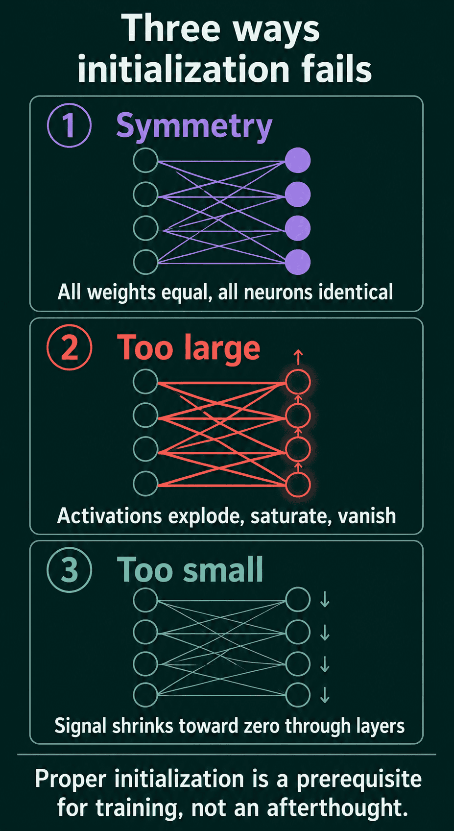
The symmetry problem: why weights cannot all start at zero
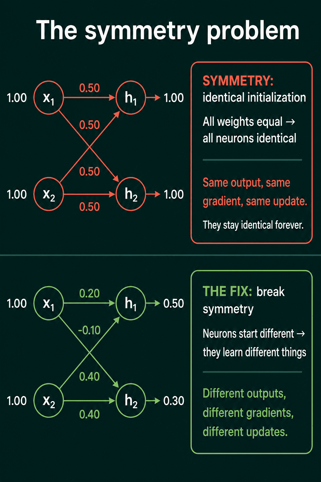
If every weight in a layer starts at the same value, every neuron in that layer computes the same output. They then receive the same gradient, get the same update, and are still identical after the step. This repeats at every step, so a hidden layer of 512 neurons behaves like one neuron copied 512 times.
The code below starts every weight and bias of a small network at 0.5 and trains it for 100 steps.
1import torch
2import torch.nn as nn
3
4torch.manual_seed(0)
5model = nn.Sequential(nn.Linear(3, 4), nn.Tanh(), nn.Linear(4, 1))
6for p in model.parameters():
7    nn.init.constant_(p, 0.5)  # every weight and bias starts at 0.5
8
9x = torch.randn(8, 3)
10y = torch.randn(8, 1)
11opt = torch.optim.SGD(model.parameters(), lr=0.1)
12for _ in range(100):
13    loss = ((model(x) - y) ** 2).mean()
14    opt.zero_grad()
15    loss.backward()
16    opt.step()
17
18print(model[0].weight)
The four rows of the first layer's weight matrix, one per hidden neuron, are still identical after training:
1tensor([[0.1739, 0.7184, 0.3469],
2        [0.1739, 0.7184, 0.3469],
3        [0.1739, 0.7184, 0.3469],
4        [0.1739, 0.7184, 0.3469]], requires_grad=True)
The weights moved, and they moved together. Starting the weights at random values fixes this, because each neuron then computes something different from the first step and gets its own gradient.
Weights too large or too small
Random weights fix symmetry, but the scale of the random values still decides what happens to the signal.
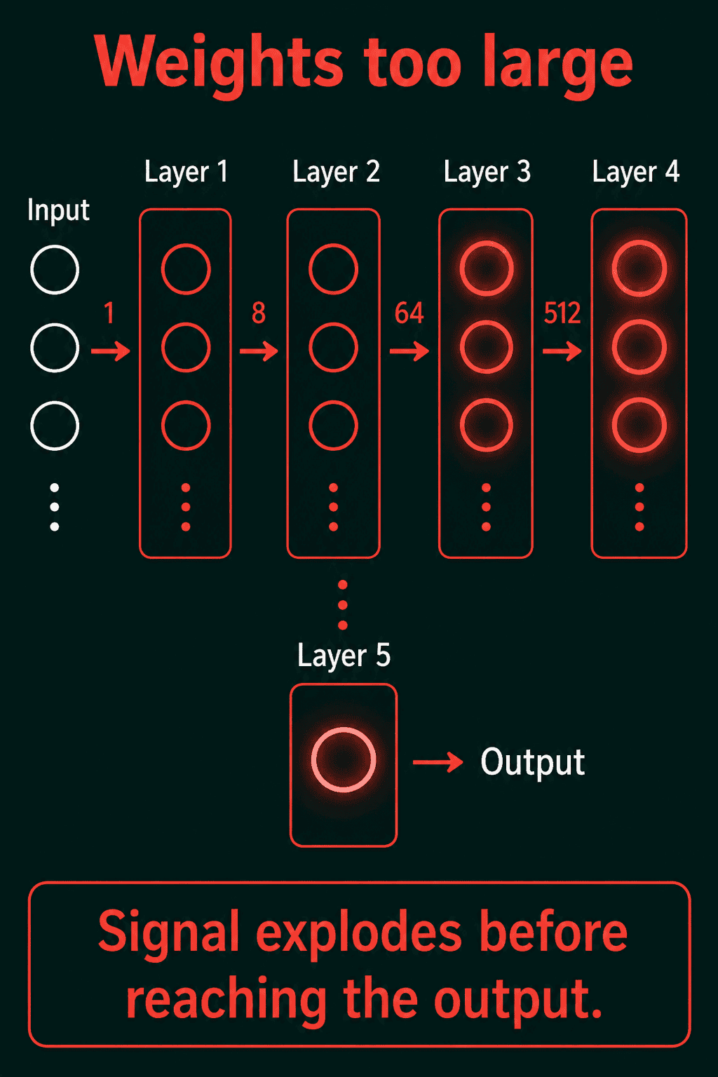
If the weights are too large, each layer multiplies the size of its input up. For tanh or sigmoid, the weighted sums land far from zero where the function is flat, so the outputs sit at the ends of the range and the gradient through them is close to zero. This is called saturation. For ReLU, which has no upper limit, the outputs grow layer after layer until they overflow or training diverges.
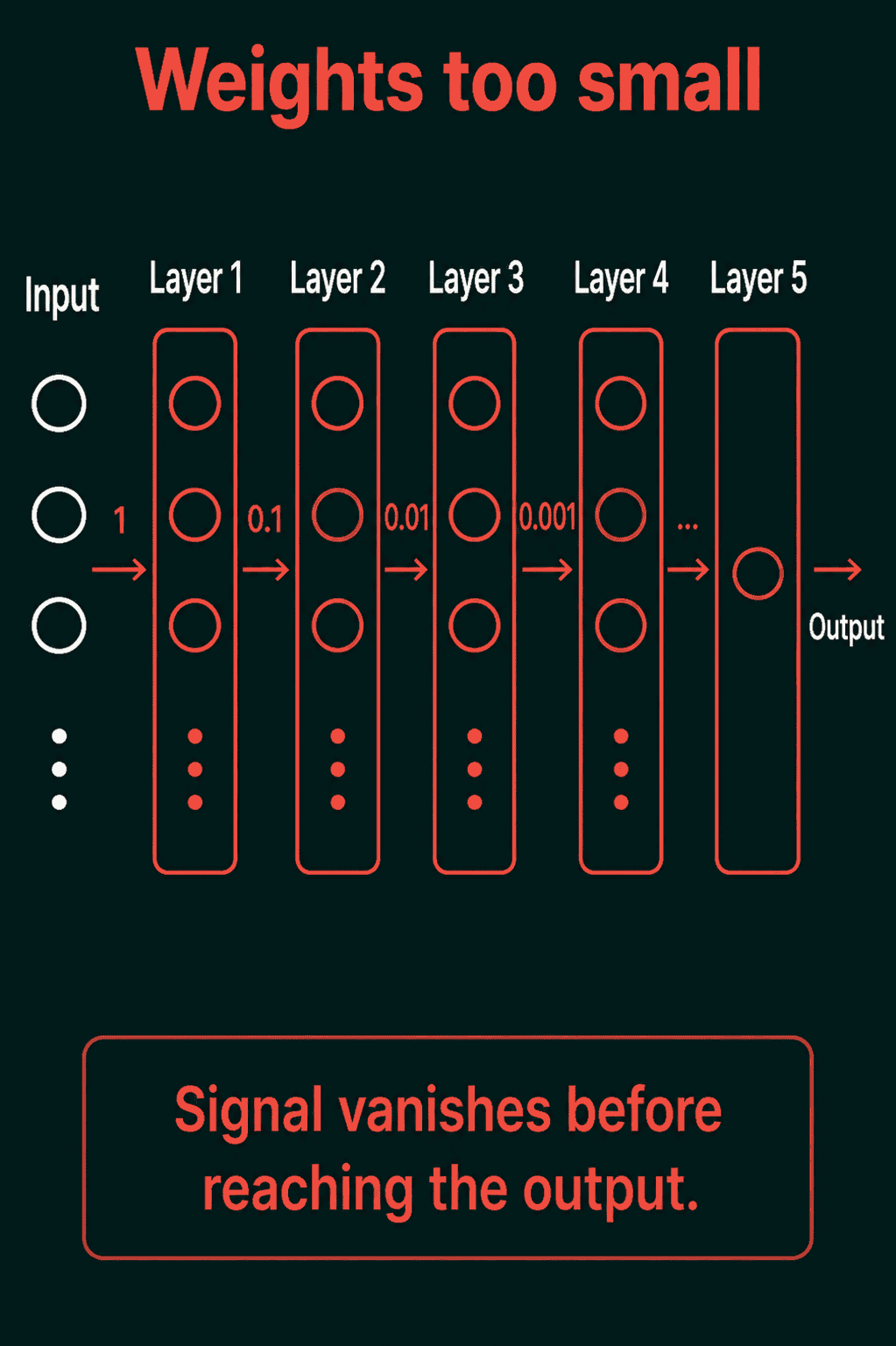
If the weights are too small, each layer multiplies the size of its input down. After a few layers the outputs are close to zero, and the gradients flowing back are close to zero too, so the early layers barely update.
The goal: keep the variance the same at every layer
The variance of a set of numbers is the average squared distance from their mean, a measure of how spread out they are. Initialization schemes pick the weight variance so that the variance of each layer's outputs stays close to the variance of its inputs.
Write $h$ for one output of a layer, $x$ for its inputs, $w$ for its weights, and $n_{in}$ for the number of inputs (the layer's fan-in). When the weights and inputs are independent with mean zero, and there is no activation yet:
$$\text{Var}(h) = n_{in} \cdot \text{Var}(w) \cdot \text{Var}(x)$$
To keep $\text{Var}(h)$ equal to $\text{Var}(x)$, the weight variance has to be $\text{Var}(w) = 1/n_{in}$. A wider layer sums more inputs, so each weight has to be smaller to keep the total the same size.
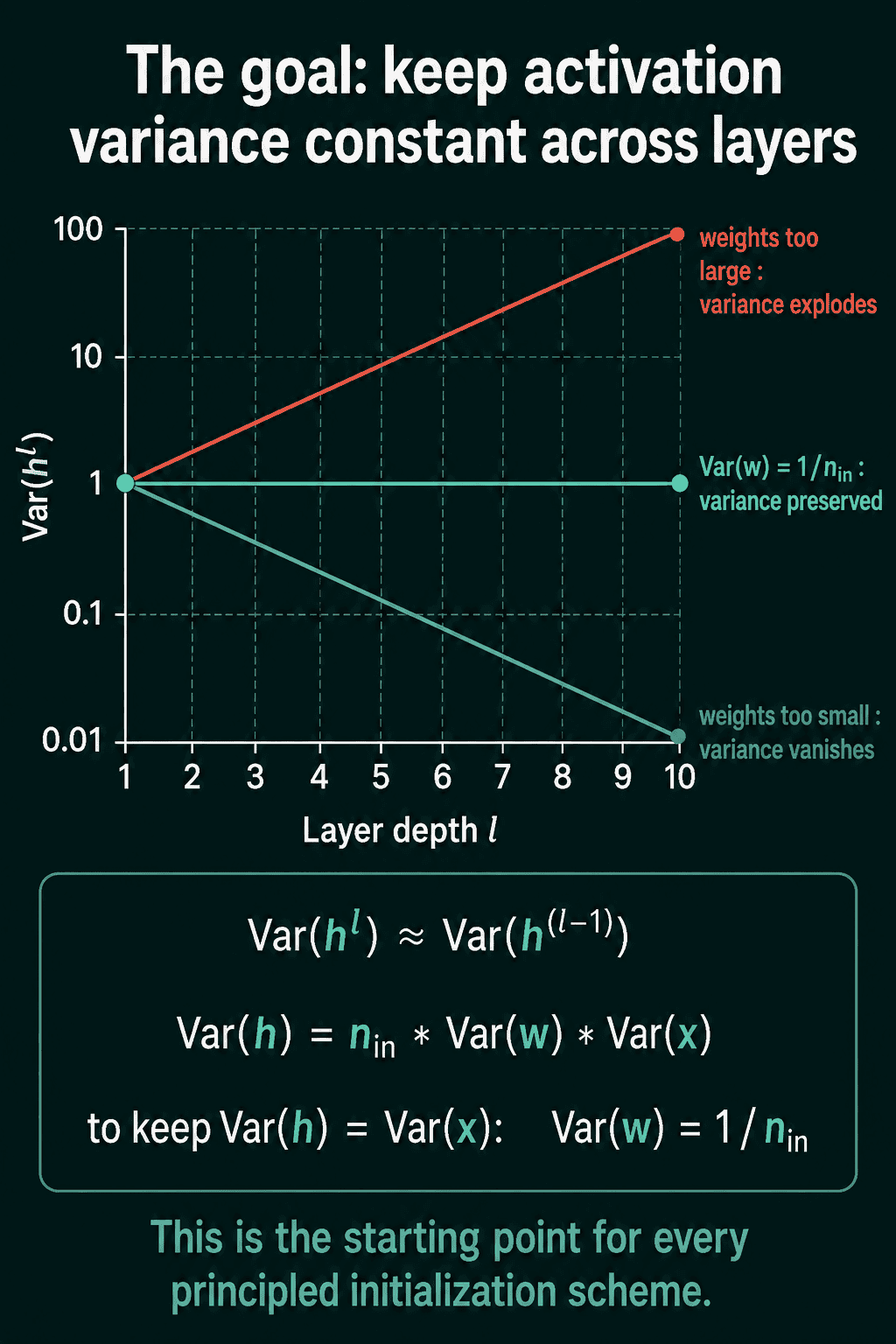
Xavier and Kaiming initialization both start from this equation and adjust it for the activation function.
Xavier (Glorot) initialization for tanh and sigmoid
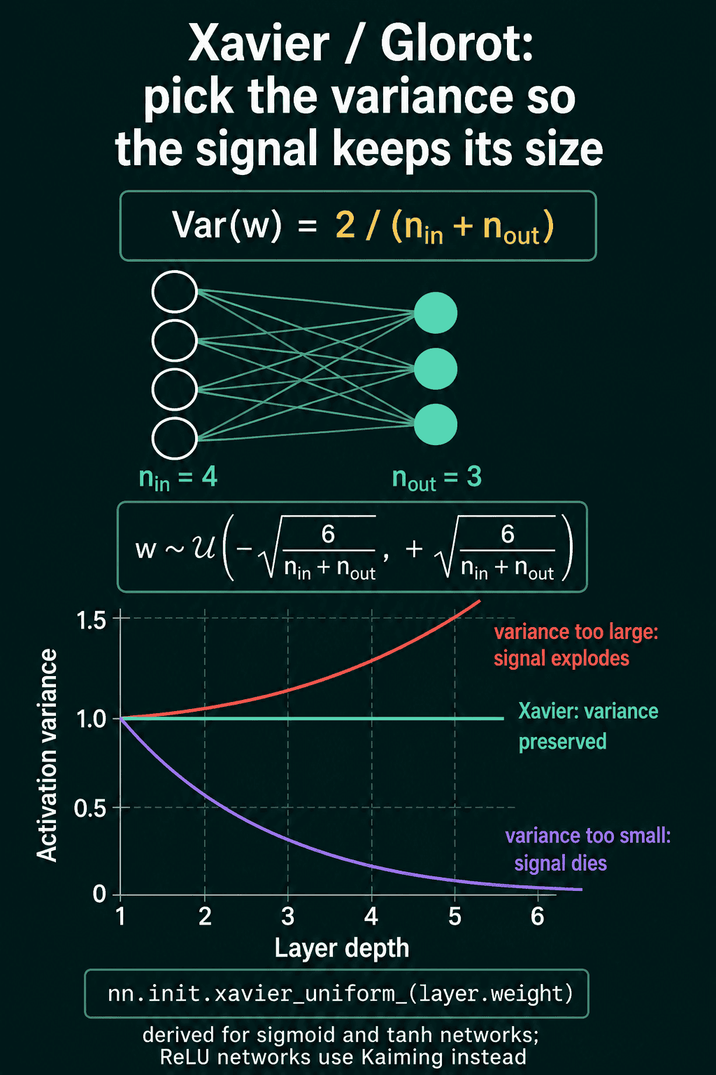
Xavier initialization, also called Glorot initialization, balances the forward pass and backpropagation. Keeping the forward outputs stable needs $1/n_{in}$, keeping the gradients stable on the way back needs $1/n_{out}$ (where $n_{out}$ is the number of outputs, the fan-out), and Xavier uses a compromise between the two:
$$\text{Var}(w) = \frac{2}{n_{in} + n_{out}}$$
The derivation assumes the activation function is roughly linear and symmetric around zero, which holds for tanh and sigmoid near zero. PyTorch has a normal version, nn.init.xavier_normal_, and a uniform version, nn.init.xavier_uniform_, which draws from a range with the same variance.
Kaiming (He) initialization for ReLU
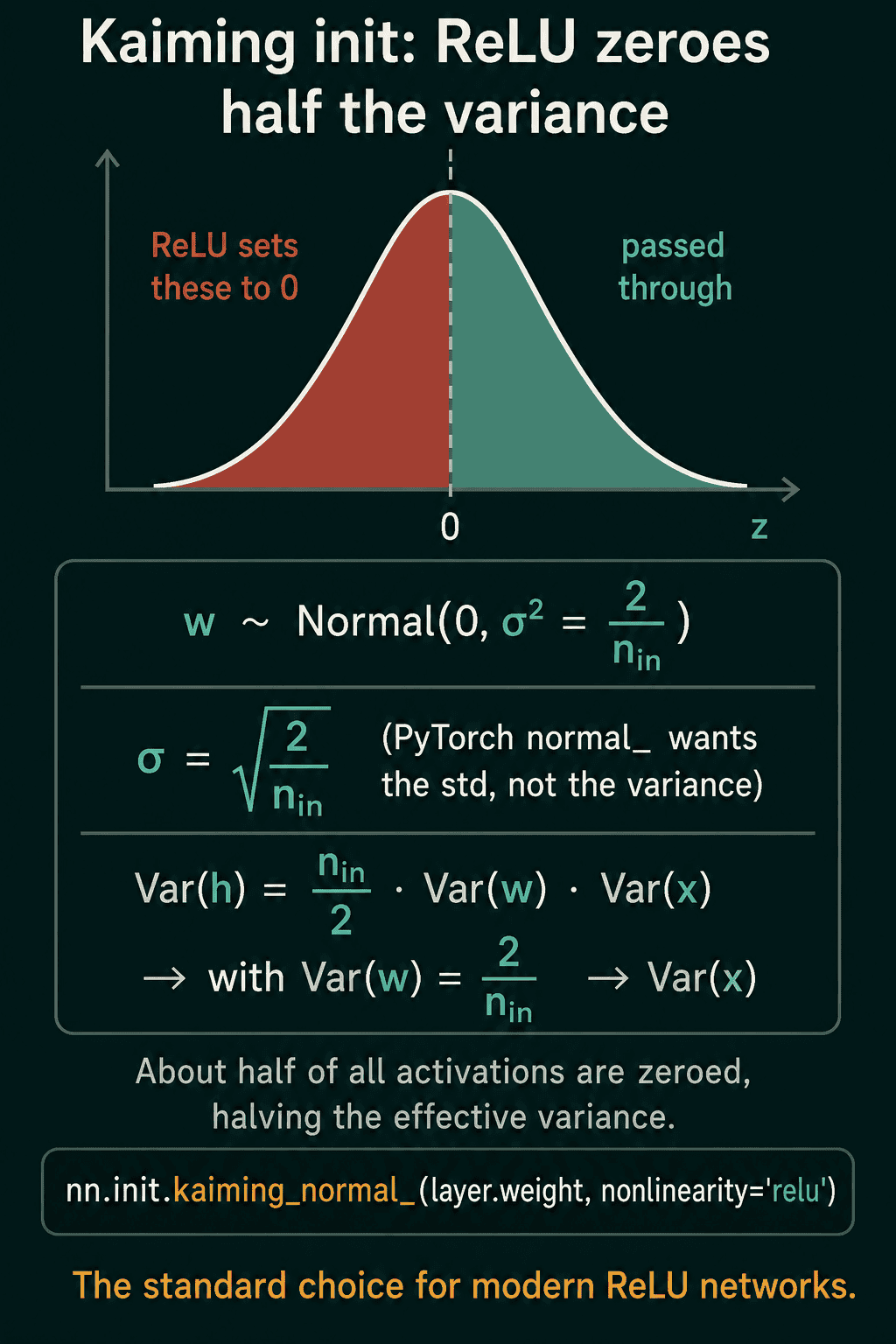
ReLU sets every negative input to zero. When the weighted sums are centered on zero, about half of them are negative, so ReLU zeroes about half the values and the variance after the activation is about half of what went in. Xavier does not account for that, so a ReLU network initialized with Xavier loses signal at every layer.
Kaiming initialization, also called He initialization, doubles the weight variance to make up for the half that ReLU removes:
$$w \sim \mathcal{N}\left(0, \frac{2}{n_{in}}\right)$$
This reads as: draw each weight from a normal distribution with mean 0 and variance $2/n_{in}$. The standard deviation is $\sqrt{2/n_{in}}$, and that is the number PyTorch's normal_ expects, not the variance.
What each scheme does to a 10-layer network
The experiment below passes 1,000 random inputs through 10 layers of width 512 and reports the standard deviation of the last layer's output (the square root of the variance, in the same units as the values). For tanh it also reports the share of outputs above 0.99 in size, which is how saturated the layer is.
1import torch
2import torch.nn as nn
3
4torch.manual_seed(0)
5
6def run(init, act, depth=10, width=512):
7    """Push one batch through `depth` layers, return the last layer's output."""
8    h = torch.randn(1000, width)
9    for _ in range(depth):
10        layer = nn.Linear(width, width, bias=False)
11        init(layer.weight)
12        h = act(layer(h))
13    return h
14
15inits = {
16    "std 1.0": lambda w: nn.init.normal_(w, std=1.0),
17    "std 0.01": lambda w: nn.init.normal_(w, std=0.01),
18    "Xavier": nn.init.xavier_normal_,
19    "Kaiming": lambda w: nn.init.kaiming_normal_(w, nonlinearity="relu"),
20}
21
22for name, init in inits.items():
23    h = run(init, torch.tanh)
24    saturated = (h.abs() > 0.99).float().mean().item()
25    print(f"tanh {name:9s} std {h.std().item():.3g}  saturated {saturated:.0%}")
26for name, init in inits.items():
27    h = run(init, torch.relu)
28 print(f"relu {name:9s} std {h.std().item():.3g}")1tanh std 1.0 std 0.982 saturated 91%
2tanh std 0.01 std 3.31e-07 saturated 0%
3tanh Xavier std 0.228 saturated 0%
4tanh Kaiming std 0.552 saturated 0%
5relu std 1.0 std 7.71e+11
6relu std 0.01 std 9.39e-09
7relu Xavier std 0.0259
8relu Kaiming std 0.828With a standard deviation of 1.0, 91% of the tanh outputs are saturated and the ReLU outputs reach about $10^{11}$. With 0.01, both shrink to almost nothing. For ReLU, Kaiming keeps the output at a similar scale to the input after 10 layers, while Xavier shrinks it by about 40 times. For tanh, Xavier avoids saturation, though the signal still shrinks slowly because tanh pulls values toward zero at each layer.
Orthogonal initialization
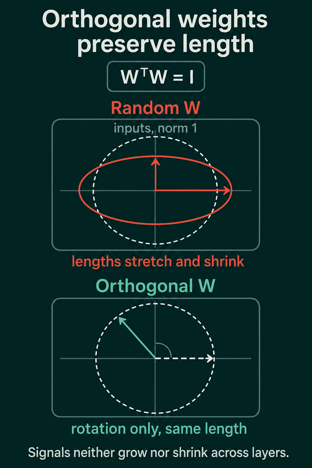
An orthogonal matrix is a square matrix $W$ with $W^\top W = I$, where $I$ is the identity matrix. Multiplying a vector by an orthogonal matrix rotates or reflects it without changing its length, so a layer with orthogonal weights neither grows nor shrinks its input.
This is most useful in recurrent neural networks (RNNs), which apply the same weight matrix once per step of a sequence, so a small stretch per step compounds over hundreds of steps. PyTorch builds a random orthogonal matrix with nn.init.orthogonal_(layer.weight), and for a non-square weight it makes the rows or the columns orthonormal, whichever fits the shape.
Weight initialization in PyTorch
nn.Linear and nn.Conv2d already initialize their weights with a uniform distribution scaled by the fan-in, so a small ReLU network often trains fine without any extra code. That default is not exactly the Kaiming formula above, though. It draws from a range of $\pm 1/\sqrt{n_{in}}$, which gives a smaller variance. When the initialization is part of what you are testing, or the network is deep, call the scheme you want after building the model:
1import torch.nn as nn
2
3def init_weights(module):
4    """He init for every Linear layer, biases at zero."""
5    if isinstance(module, nn.Linear):
6        nn.init.kaiming_normal_(module.weight, nonlinearity="relu")
7        nn.init.zeros_(module.bias)
8
9model = nn.Sequential(
10    nn.Linear(784, 256), nn.ReLU(),
11    nn.Linear(256, 256), nn.ReLU(),
12    nn.Linear(256, 10),
13)
14model.apply(init_weights)
15print(model[0].weight.std().item())
This prints about 0.05, close to $\sqrt{2/784} \approx 0.0505$. model.apply calls the function on every submodule, so the same line works for a network of any depth. If training fails right at the start, the first thing to check is whether the output scale of each layer stays near the input scale, as in the experiment above.
When to use which initialization
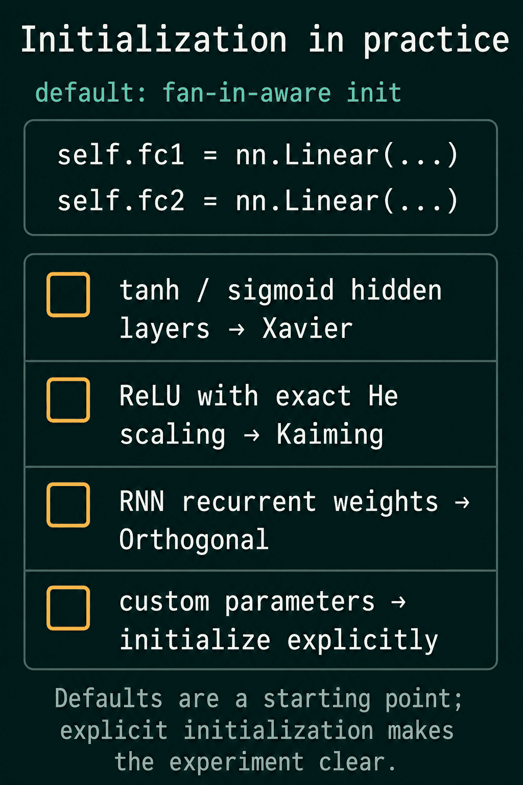
| Network | Initialization | PyTorch call |
|---|---|---|
| tanh or sigmoid hidden layers | Xavier | xavier_uniform_ |
| ReLU hidden layers | Kaiming | kaiming_normal_ |
| RNN recurrent weights | orthogonal | orthogonal_ |
| custom module parameters | pick one on purpose | any of the above |
Common mistakes
- Initializing all weights to zero or one constant. Every neuron in the layer stays identical, as the symmetry experiment showed. Biases can start at zero, since random weights already make the neurons differ.
- Passing the variance where PyTorch expects the standard deviation.
nn.init.normal_(w, std=2 / n_in)uses $2/n_{in}$ as the standard deviation, which is far too small. The Kaiming value isstd=(2 / n_in) ** 0.5. - Using Xavier on a deep ReLU network. ReLU halves the variance at each layer, and Xavier does not correct for it, so the signal shrinks with depth.
- Forgetting custom parameters. A tensor wrapped in
nn.Parameterinside your own module is not touched bynn.Linear's default, so it keeps whatever values you created it with.
Related concepts
Activation functions decide which initialization fits: tanh and sigmoid pair with Xavier, ReLU and its variants with Kaiming. Backpropagation is where a bad initialization shows up, since it multiplies the gradient by every layer's weights on the way back. Vanishing and exploding gradients are the training-time version of the too-small and too-large problems above, and a common fix for them is gradient clipping. Dead ReLU neurons, units that output zero for every input, are more likely when the starting scale is wrong.
QuiddityML teaches weight initialization in Unit 2 of the ML Foundation track, where the Kaiming exercises include matching the formula to its code, spotting the bug in an initializer that uses $1/n_{in}$ where ReLU needs $2/n_{in}$, and writing kaiming_normal_ from scratch (quiddityml.com).