29 September 2026 · 7 min read

Vanishing and exploding gradients, and how gradient clipping helps

Vanishing and exploding gradients happen when the training signal shrinks to almost nothing or grows out of control as it passes back through a deep network. This post shows why both happen, how to measure them in PyTorch, and how ReLU, good initialization, and gradient clipping help.

A vanishing gradient is a training signal that shrinks toward zero as it travels back through a deep network, so the early layers barely learn. An exploding gradient is the opposite: the signal grows as it travels back, the weights get huge updates, and the loss jumps around or turns into NaN. Both come from the same multiplication, and both get worse as networks get deeper.

What a gradient is and how it travels back

A neural network is trained by gradient descent. The network makes predictions, a loss (one number that measures how wrong those predictions are) is computed, and each weight is moved a small step in the direction that lowers the loss. The gradient of the loss with respect to a weight says how much the loss changes when that weight changes, and it sets the size and direction of that weight's step.

The gradients are computed by backpropagation, which starts at the loss and works backward one layer at a time. Each layer takes the gradient it receives from the layer above, multiplies it by its own local gradient (the derivative of that layer's output with respect to its input), and passes the result down. The gradient that reaches layer 1 of a 10-layer network is the output gradient multiplied by nine local gradients in a row.

Why gradients vanish

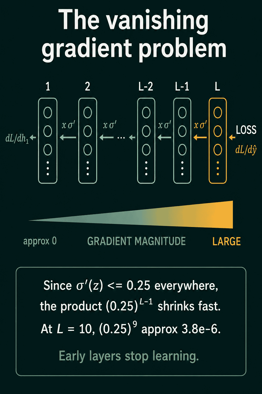
Take a network whose hidden layers use the sigmoid activation, $\sigma(z) = 1/(1 + e^{-z})$, which squashes any number into the range 0 to 1. Its derivative $\sigma'(z)$ is at most 0.25, reached at $z = 0$, and smaller everywhere else.

Write $\mathcal{L}$ for the loss, $\hat{y}$ for the network's output, $\mathbf{h}_1$ for the output of layer 1, and $L$ for the number of layers. Ignoring the weights for a moment, the gradient that reaches layer 1 is roughly the output gradient times one sigmoid derivative per layer:

$$\frac{\partial \mathcal{L}}{\partial \mathbf{h}1} \approx \frac{\partial \mathcal{L}}{\partial \hat{y}} \cdot \prod{l=2}^{L} \sigma'(z_l)$$

The $\prod$ symbol means multiply all the terms together. Since each $\sigma'(z_l)$ is at most 0.25, the product is at most $0.25^{L-1}$. At $L = 10$ that is $0.25^9 \approx 3.8 \times 10^{-6}$, so the gradient reaching the first layer is at least 260,000 times smaller than the one at the output. The later layers train, and the early layers stay close to their starting values.

The vanishing gradient problem: the gradient is multiplied by σ' at each layer from L back to 1, shrinking from large at the loss to about 0 at layer 1, with the note that at L = 10, 0.25 to the power 9 is about 3.8e-6.

Why ReLU helps

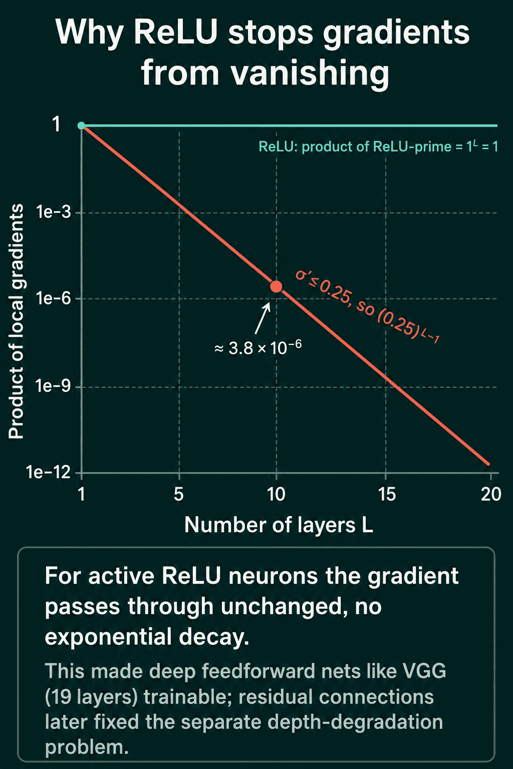
ReLU, $\text{ReLU}(z) = \max(0, z)$, keeps positive inputs and sets negative ones to 0. Its derivative is 1 for positive inputs and 0 for negative ones. For a neuron with a positive input, multiplying by 1 leaves the gradient unchanged, so a chain of ReLU layers does not shrink the gradient the way a chain of sigmoids does.

$$\prod_{l=1}^{L} \text{ReLU}'(z_l) = 1^L = 1 \quad \text{(active neurons)}$$

Switching from sigmoid to ReLU is a large part of why networks with 10 to 20 layers became trainable. The derivative of 0 for negative inputs has its own cost, though. A neuron whose input is negative for every example passes no gradient back at all, and it stops learning. This is called a dead ReLU.

Product of local gradients against the number of layers on a log scale: the ReLU line stays at 1, while the sigmoid line falls along 0.25 to the power L minus 1, reaching about 3.8 × 10^-6 at 10 layers and about 1e-12 at 20.

Much deeper networks, with 50 or more layers, also add residual connections, which add a layer's input directly to its output so the gradient has a path around the layer. Recurrent neural networks, which apply the same weight matrix at every step of a sequence, get vanishing gradients over long sequences even with ReLU. Architectures such as the LSTM were built to handle that case.

Why gradients explode

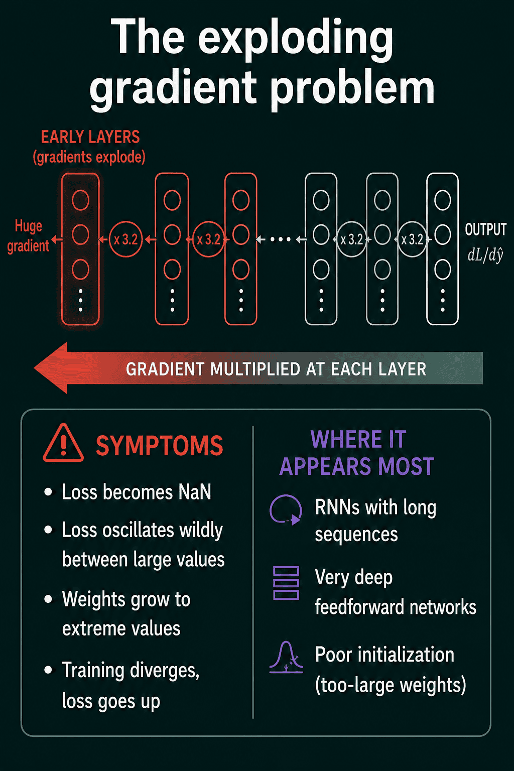
The same product can grow instead of shrink. The weights are part of each layer's local gradient too, and if the weights are large, each layer multiplies the gradient by a number above 1. Ten layers that each multiply by 3.2 turn a gradient of 1 into about 110,000.

When the gradient explodes, the weights get enormous updates and jump to extreme values. The symptoms are easy to spot in a training log:

The loss becomes NaN or inf.
The loss swings between large values instead of going down.
The weights grow into the thousands or millions.
The loss goes up over training instead of down.

Exploding gradients show up most in recurrent networks trained on long sequences, in very deep feedforward networks, and in networks whose initial weights are too large.

The exploding gradient problem: the gradient is multiplied by 3.2 at each layer on its way back, becoming huge at the early layers, with the symptoms (loss becomes NaN, loss oscillates, weights grow to extreme values, training diverges) and where it appears most (RNNs with long sequences, very deep feedforward networks, too-large initial weights).

Measuring gradients layer by layer in PyTorch

After loss.backward(), every weight tensor has a .grad attribute holding its gradient. Its norm (the square root of the sum of its squared entries, one number for the size of the whole tensor) shows how much signal that layer received. The script below builds three 10-layer networks and prints the gradient norm of the first and last hidden layers.

1import torch
2import torch.nn as nn
3 
4torch.manual_seed(0)
5WIDTH = 256
6 
7def make_net(act, init, depth=10):
8    """`depth` hidden Linear + activation layers, then a 1-unit output layer."""
9    layers = []
10    for _ in range(depth):
11        linear = nn.Linear(WIDTH, WIDTH)
12        init(linear.weight)
13        nn.init.zeros_(linear.bias)
14        layers += [linear, act()]
15    layers.append(nn.Linear(WIDTH, 1))
16    return nn.Sequential(*layers)
17 
18def grad_norms(net):
19    """Gradient norm of each hidden layer's weight after one backward pass."""
20    x = torch.randn(64, WIDTH)
21    loss = net(x).pow(2).mean()
22    loss.backward()
23    hidden = [m for m in net if isinstance(m, nn.Linear)][:-1]
24    return [m.weight.grad.norm().item() for m in hidden]
25 
26xavier = nn.init.xavier_normal_
27kaiming = lambda w: nn.init.kaiming_normal_(w, nonlinearity="relu")
28too_big = lambda w: nn.init.normal_(w, std=0.2)
29 
30for name, net in [
31    ("sigmoid, Xavier", make_net(nn.Sigmoid, xavier)),
32    ("ReLU, Kaiming", make_net(nn.ReLU, kaiming)),
33    ("ReLU, std 0.2", make_net(nn.ReLU, too_big)),
34]:
35    g = grad_norms(net)
36    print(f"{name:16s} layer 1: {g[0]:.1e}   layer 10: {g[-1]:.1e}")

1sigmoid, Xavier  layer 1: 3.2e-07   layer 10: 6.9e-01
2ReLU, Kaiming    layer 1: 1.2e+00   layer 10: 8.3e+00
3ReLU, std 0.2    layer 1: 4.1e+06   layer 10: 2.3e+07

In the sigmoid network, layer 1 gets a gradient about two million times smaller than layer 10, which is the vanishing gradient. The ReLU network with Kaiming initialization (random starting weights scaled so each layer keeps the signal the same size) keeps both layers within a factor of about 7. The same ReLU network with weights drawn at a standard deviation of 0.2, about 2.3 times the Kaiming value for this width, has gradients in the millions, which is the exploding gradient. Printing these norms every few hundred steps is a quick way to see which problem a stuck run has.

Gradient clipping

Gradient clipping caps the size of the gradient before the optimizer uses it. The common version is clipping by norm: if the norm of all gradients together is above a threshold $\gamma$, every gradient is scaled down by the same factor so the total norm equals $\gamma$. Writing $\mathbf{g}$ for all the gradients stacked into one vector:

$$\mathbf{g} \leftarrow \frac{\gamma}{\max(|\mathbf{g}|, \gamma)} , \mathbf{g}$$

When $|\mathbf{g}|$ is below $\gamma$, the fraction is 1 and nothing changes. When it is above, every entry shrinks by the same factor, so the update still points in the same direction and only its length is capped.

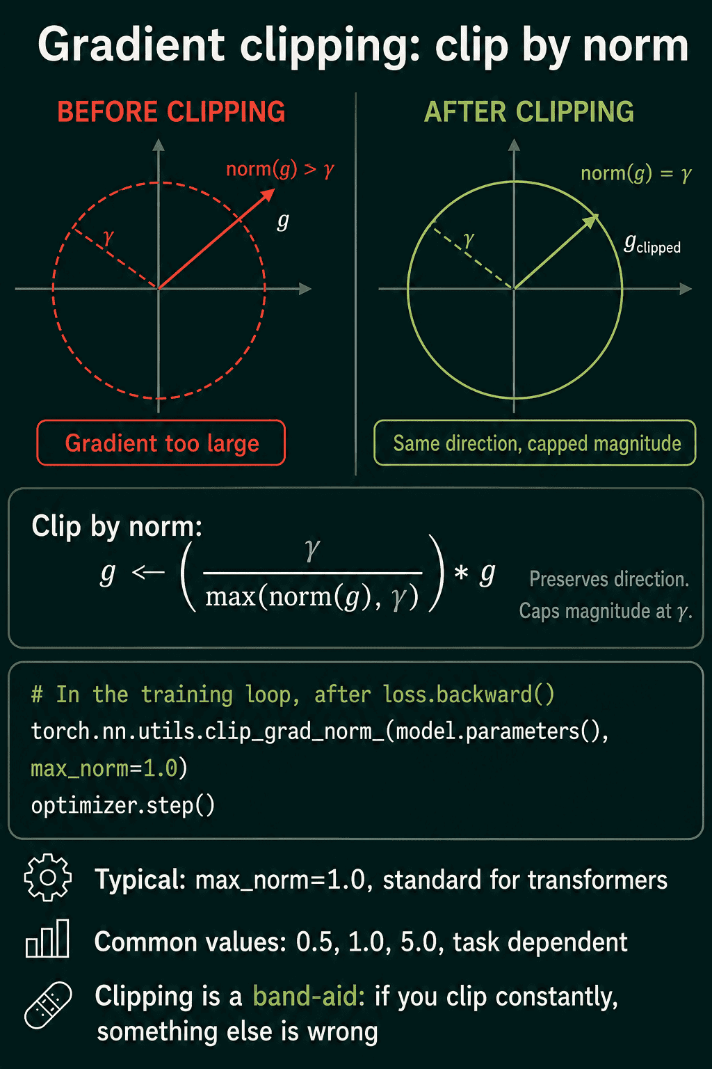
Gradient clipping by norm: before clipping the gradient vector g extends past the circle of radius γ, and after clipping it points the same way with length γ, next to the formula and the PyTorch call clip_grad_norm_(model.parameters(), max_norm=1.0) placed before optimizer.step().

In PyTorch, clipping goes between loss.backward(), which computes the gradients, and optimizer.step(), which uses them. clip_grad_norm_ also returns the total norm before clipping, which is worth logging.

1import torch
2import torch.nn as nn
3 
4torch.manual_seed(0)
5model = nn.Linear(4, 1)
6x = torch.randn(16, 4) * 100  # inputs far too large, so the gradient is huge
7y = torch.randn(16, 1)
8 
9loss = ((model(x) - y) ** 2).mean()
10loss.backward()
11 
12before = torch.nn.utils.clip_grad_norm_(model.parameters(), max_norm=1.0)
13after = torch.cat([p.grad.flatten() for p in model.parameters()]).norm()
14print(f"norm before: {before:.1f}   norm after: {after:.3f}")

1norm before: 10564.1   norm after: 1.000

A max_norm of 1.0 is a common default for transformer training, and some tasks use 0.5 or 5.0. PyTorch also has clip_grad_value_, which caps each entry on its own at a value such as 1.0. That changes the direction of the gradient, because large entries are cut and small ones are not, so clipping by norm is the usual choice.

When to use gradient clipping, and when to look elsewhere

Clipping is standard for recurrent networks and transformers, where a single bad batch can produce a gradient spike that undoes hours of training. It costs one line and does nothing when gradients are already small.

If the logged norm is above the threshold on most steps, though, clipping is covering up another problem. Lower the learning rate, check the weight initialization, and look at the data for extreme values before relying on clipping. Vanishing gradients get no help from clipping at all, since clipping only shrinks gradients. For those, the usual fixes are ReLU-family activations, Kaiming initialization, residual connections, and normalization layers.

Common mistakes

Clipping before loss.backward() or after optimizer.step(). Before backward there are no new gradients to clip, and after step the update has already been applied. Clip between the two.
Clipping each parameter tensor separately in a loop. Calling clip_grad_norm_ on one layer at a time caps each layer's norm on its own, which changes the direction of the overall update. Pass model.parameters() in one call.
Treating a NaN loss as a data bug first. A gradient that explodes over a few steps produces NaN too. Log the gradient norm and check whether it grew before the NaN appeared.
Adding more sigmoid layers to a network that already trains badly. The extra layers add more factors of at most 0.25 to the product, so the early layers get even less signal.

Backpropagation is where both problems come from, since it multiplies local gradients layer by layer. Weight initialization sets the starting scale of that product, and Kaiming initialization for ReLU is a common first fix. Activation functions set the local gradients: sigmoid and tanh shrink them, ReLU keeps them at 1 for active neurons. Dead ReLU neurons are the cost of ReLU's zero derivative for negative inputs. The learning rate multiplies every gradient before the update, so a lower learning rate is often the fix when clipping triggers on most steps.

QuiddityML teaches vanishing gradients, exploding gradients, and gradient clipping as three concepts in Unit 2 of the ML Foundation track, and the exercises include writing the global gradient-norm check, ordering the lines of a training loop with clipping, and spotting a clip placed before loss.backward() (quiddityml.com).