By Sagi Shaier · 16 October 2026 · 6 min read
The Gaussian (normal) distribution explained
What the mean and standard deviation do to the bell curve, how to standardize any Gaussian to z-scores, and why code works with the log-density, with every step checked in PyTorch.
The Gaussian distribution, also called the normal distribution, is the bell-shaped distribution of a continuous quantity that is built from many small independent effects. Adult heights, measurement noise and the errors of a regression model are often modeled this way. It is the continuous distribution ML uses most often, and it is the distribution behind the mean squared error loss.
Density, not probability
A continuous quantity like height can take any value, so the probability of one exact value, like exactly 180.000 cm, is 0. A continuous distribution gives a density instead, a curve whose area over a range is the probability of landing in that range. The total area under the curve is 1. A density value on its own is not a probability, and it can be larger than 1.
The Gaussian density formula
The Gaussian has two parameters. The mean $\mu$ (mu) is the center of the curve. The variance $\sigma^2$ (sigma squared) sets how wide it is, and its square root $\sigma$ is the standard deviation, measured in the same units as the data. The density at a value $x$ is:
$$p(x) = \frac{1}{\sqrt{2\pi\sigma^{2}}}\exp\!\left(-\frac{(x-\mu)^{2}}{2\sigma^{2}}\right)$$
$\exp(a)$ means $e^a$, with $e \approx 2.718$. Each part has one job:
- $\mu$ slides the peak along the number line.
- $\sigma^2$ sets the width.
- $1/\sqrt{2\pi\sigma^2}$ in front is the constant that keeps the total area at 1 as the curve gets wider or narrower.
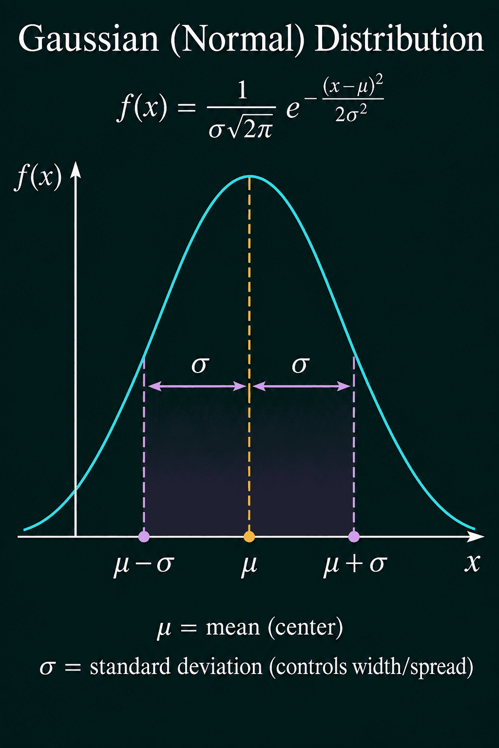
The picture writes the constant as $1/(\sigma\sqrt{2\pi})$, which is the same number, since $\sqrt{2\pi\sigma^2} = \sigma\sqrt{2\pi}$.
A worked example with heights
Take heights with $\mu = 170$ cm and $\sigma = 10$ cm. At the peak, $x = 170$, the exponent is 0 and $e^0 = 1$, so the density is only the constant:
$$p(170) = \frac{1}{10\sqrt{2\pi}} = 0.0399$$
One standard deviation away, at $x = 180$, the exponent is $-(10^2)/(2 \times 10^2) = -0.5$:
$$p(180) = 0.0399 \times e^{-0.5} = 0.0399 \times 0.607 = 0.0242$$
The density depends on $x$ only through the squared distance $(x - \mu)^2$. So 160 and 180 get the same density, and the curve is symmetric around $\mu$. The squared distance also makes the density fall off fast away from the center. Relative to the peak, it is 0.61 at one standard deviation, 0.14 at two and 0.011 at three.
The constant also explains the height of the peak. Halve $\sigma$ to 5 and the constant doubles to 0.0798. The curve gets twice as tall and half as wide, and its area stays 1. With $\sigma = 0.1$ the peak density is about 3.99, a density above 1, which is fine for a density.
The standard normal and z-scores
Set $\mu = 0$ and $\sigma = 1$ and the formula becomes the standard normal density, often written $\phi(z)$ (phi):
$$\phi(z) = \frac{1}{\sqrt{2\pi}}e^{-z^{2}/2}$$
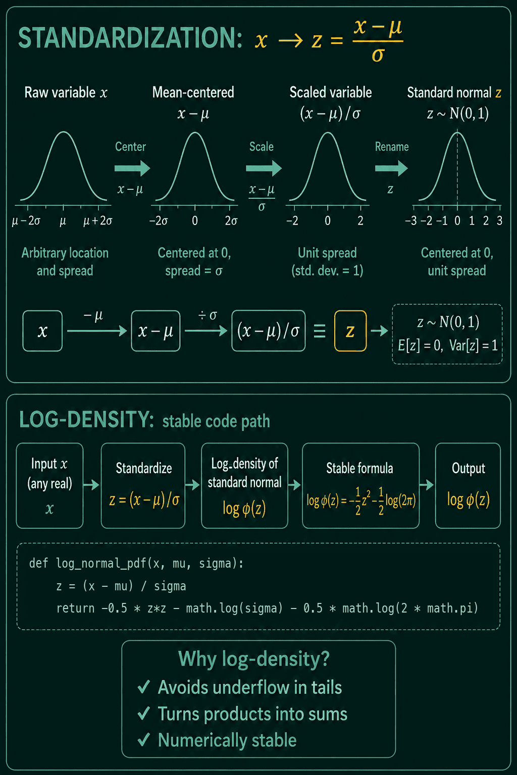
The notation $N(\mu, \sigma^2)$ means "a Gaussian with mean $\mu$ and variance $\sigma^2$", so the standard normal is $N(0, 1)$. Any Gaussian turns into the standard normal by standardizing: subtract the mean, then divide by the standard deviation.
$$z = \frac{x - \mu}{\sigma}$$
The result $z$ is called a z-score, and it counts how many standard deviations $x$ sits from the mean. For the heights, 185 cm becomes $z = (185 - 170)/10 = 1.5$ and 150 cm becomes $z = -2$. Because of this, one table of standard-normal values serves every Gaussian. A quantile is the value below which a given share of the probability lies, and the quantiles of any Gaussian are the standard-normal quantiles scaled by $\sigma$ and shifted by $\mu$.
Why code uses the log-density
Training code rarely evaluates the density itself. A dataset's likelihood is the product of the densities of all its points, and a product of hundreds of small numbers underflows: it rounds to exactly 0 in floating point. Take the log and the product becomes a sum. The log of the Gaussian density is:
$$\log p(x) = -\frac{(x-\mu)^{2}}{2\sigma^{2}} - \log \sigma - \tfrac{1}{2}\log(2\pi)$$
The exponential is gone, so each term is an ordinary number. For $x = 180$ with $\mu = 170$ and $\sigma = 10$, the three terms are $-0.5$, $-\log 10 = -2.303$ and $-0.919$, which add up to $-3.722$. And $e^{-3.722} = 0.0242$, the same density as before.
Log-likelihood and squared error
Look at the first term of the log-density: a squared error $(x - \mu)^2$ divided by $2\sigma^2$. Add up the log-densities of a dataset with $\sigma$ fixed, and the other two terms are the same constant for every choice of $\mu$. So the $\mu$ with the highest log-likelihood is the $\mu$ with the smallest total squared error. Maximizing a Gaussian log-likelihood at fixed $\sigma$ is the same as minimizing squared error. So training a regression model with mean squared error gives the same answer as fitting the mean of a Gaussian with a fixed $\sigma$.
The Gaussian in PyTorch
The density formula written out by hand matches torch.distributions.Normal:
1import math
2import torch
3from torch.distributions import Normal
4
5def gaussian_pdf(x, mu, sigma):
6    return torch.exp(-(x - mu) ** 2 / (2 * sigma ** 2)) / math.sqrt(2 * math.pi * sigma ** 2)
7
8x = torch.tensor([170.0, 180.0, 190.0, 200.0])
9print(gaussian_pdf(x, 170.0, 10.0))
10print(Normal(170.0, 10.0).log_prob(x).exp())
11# tensor([0.0399, 0.0242, 0.0054, 0.0004])
12# tensor([0.0399, 0.0242, 0.0054, 0.0004])
Standardizing is one line:
1import torch
2
3x = torch.tensor([150.0, 165.0, 170.0, 185.0])
4z = (x - 170.0) / 10.0
5print(z)
6# tensor([-2.0000, -0.5000,  0.0000,  1.5000])
The underflow is easy to reproduce. Multiply the densities of 1000 people who are each 180 cm tall, then add their log-densities instead:
1import torch
2from torch.distributions import Normal
3
4heights = Normal(170.0, 10.0)
5x = torch.full((1000,), 180.0)
6
7print(heights.log_prob(x).exp().prod())   # product of 1000 densities
8print(heights.log_prob(x).sum())          # sum of 1000 log-densities
9# tensor(0.)
10# tensor(-3721.5237)
The product is exactly 0, so it can no longer tell one choice of $\mu$ from another. The sum is $1000 \times -3.7215$, a normal number. Finally, the squared-error connection: on the data 2, 3 and 7, scan $\mu$ from 0 to 8 and pick the best value by each measure:
1import torch
2from torch.distributions import Normal
3
4data = torch.tensor([2.0, 3.0, 7.0])
5mus = torch.linspace(0, 8, 81)
6
7sq_err = torch.stack([((data - m) ** 2).sum() for m in mus])
8log_lik = torch.stack([Normal(m, 1.0).log_prob(data).sum() for m in mus])
9
10print(mus[sq_err.argmin()].item(), mus[log_lik.argmax()].item())
11# 4.0 4.0
Both pick $\mu = 4$, the mean of the data.
When to use a Gaussian, and common mistakes
A Gaussian is a good default for a continuous quantity that can be above or below its center by similar amounts, like measurement noise or a regression error. It is a poor fit for a quantity that cannot be negative, such as a duration, because it puts some probability below zero.
- Passing the variance where the standard deviation goes.
Normal(loc, scale)takes $\sigma$ asscale, not $\sigma^2$.Normal(170.0, 100.0)is a Gaussian with a standard deviation of 100 cm. - Multiplying densities. A product over a dataset underflows to 0. Sum
log_probinstead. - Reading a density as a probability. A density of 3.99 is valid. Probabilities come from area under the curve.
- Standardizing with the wrong statistics. At test time, use the $\mu$ and $\sigma$ computed on the training data, so every input is shifted and scaled the same way.
Related concepts
Common probability distributions covers the Bernoulli, binomial, Poisson and Beta, and where the Gaussian sits among the continuous families. Maximum likelihood estimation builds on the log-likelihood shown here, and it shows where MSE and cross-entropy come from. Degrees of freedom sets the shape of Student's t, a Gaussian-like distribution with heavier tails. The multivariate Gaussian extends the same formula to vectors, with a covariance matrix in place of $\sigma^2$.
QuiddityML teaches the Gaussian as a concept in the Math track's probability unit, and the exercises on it include predicting what halving $\sigma$ does to the peak, filling in the log-density term by term and writing a standardize function from scratch.