By Sagi Shaier · 15 October 2026 · 6 min read
Bayes' theorem explained with an example
Where the formula comes from, what the prior, likelihood and posterior mean, and a spam filter example worked by hand and in PyTorch, including how the prior changes the answer.
Bayes' theorem is a formula that turns one conditional probability into its reverse: from the probability of the evidence given a cause to the probability of the cause given the evidence. The direction you can measure is often the opposite of the one you want. You can count how often spam emails contain the word "free", and what a spam filter needs is the probability that an email is spam once it sees "free". Bayes' theorem connects the two.
Conditional probability in one table
A conditional probability is the probability of one event once you know another happened. $P(B \mid A)$ is read "the probability of $B$ given $A$". Here is how a set of emails splits by two events, whether the email contains "free" and whether it is spam. Each cell is the probability that an email lands in it, and the four cells add up to 1:
| spam | not spam | |
|---|---|---|
| contains free | 0.30 | 0.10 |
| no free | 0.20 | 0.40 |
The probability of both events together, $P(\text{free}, \text{spam})$, is one cell: 0.30. This is called a joint probability. The probability of one event on its own is a row or column total. $P(\text{spam}) = 0.30 + 0.20 = 0.50$ and $P(\text{free}) = 0.30 + 0.10 = 0.40$.
A conditional probability is the joint divided by the total of the event you condition on:
$$P(\text{free} \mid \text{spam}) = \frac{P(\text{free}, \text{spam})}{P(\text{spam})} = \frac{0.30}{0.50} = 0.60$$
60% of spam emails contain "free". Turned around, $P(\text{spam} \mid \text{free}) = 0.30 / 0.40 = 0.75$, so 75% of emails with "free" are spam. The two numbers answer different questions, and Bayes' theorem gets from the first to the second.
Deriving the formula
Multiply both sides of the conditional probability formula by the denominator and you get the product rule, a joint written as a conditional times a single probability. It works in both directions:
$$P(A, B) = P(A \mid B)\,P(B)$$
$$P(A, B) = P(B \mid A)\,P(A)$$
Check both on the table, with $A$ as spam and $B$ as free: $0.75 \times 0.40 = 0.30$ and $0.60 \times 0.50 = 0.30$. Both right-hand sides equal the same joint, so they equal each other. Divide by $P(B)$ and you get Bayes' theorem:
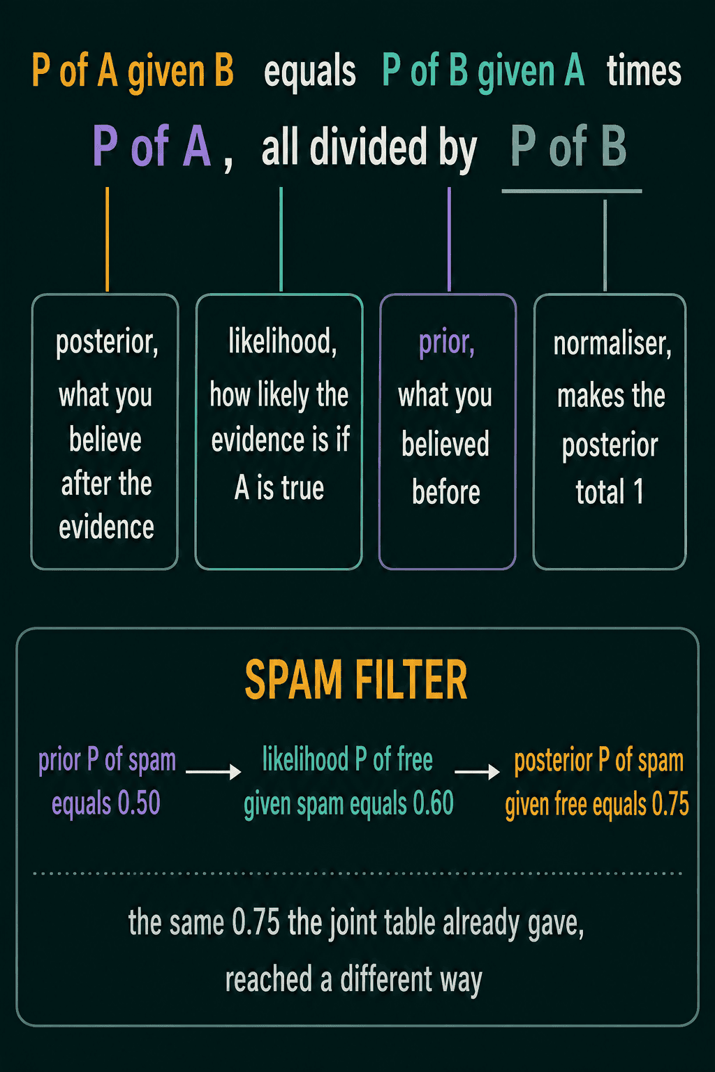
$$P(A \mid B) = \frac{P(B \mid A)\,P(A)}{P(B)}$$
It computes the probability of $A$ given $B$ from the probability of $B$ given $A$.
Prior, likelihood and posterior
Each piece of the formula has a name:
- $P(A)$ is the prior: what you believed about $A$ before seeing the evidence.
- $P(B \mid A)$ is the likelihood: how likely the evidence is if $A$ is true.
- $P(A \mid B)$ is the posterior: what you believe about $A$ after seeing the evidence.
- $P(B)$ is the normalizer, which makes the posterior probabilities of every case add up to 1.
For the spam filter, $A$ is "the email is spam" and $B$ is "the email contains free". The prior is the share of all email that is spam. The likelihood is how often spam contains "free". The posterior is the probability that this particular email is spam, now that you have seen "free" in it.
Working out the denominator
$P(B)$ is rarely handed to you directly. You can build it from the cases of $A$. An email is either spam or not spam, so every email containing "free" is in one of the two groups. Add the share of "free" emails from each group:
$$P(B) = \sum_a P(B \mid a)\,P(a)$$
The $\sum_a$ means "add up over every case $a$", here spam and not spam. Each term is the likelihood of the evidence in that case times the prior of that case. This expansion is called the law of total probability.
The spam example, step by step
Suppose you know three numbers and no table:
- the prior, $P(\text{spam}) = 0.50$
- the likelihood, $P(\text{free} \mid \text{spam}) = 0.60$
- the rate of "free" in normal email, $P(\text{free} \mid \text{not spam}) = 0.20$
First the denominator, split on spam and not spam:
$$P(\text{free}) = 0.60 \times 0.50 + 0.20 \times 0.50 = 0.40$$
Then Bayes' theorem:
$$P(\text{spam} \mid \text{free}) = \frac{0.60 \times 0.50}{0.40} = 0.75$$
Seeing "free" moves the probability of spam from 0.50 to 0.75. This is the same 0.75 you get by reading the table directly, $0.30 / 0.40$. Bayes' theorem is a route to that number when you have the likelihoods and the prior but no joint table.
How the prior changes the answer
Keep the likelihoods the same and change the prior. If only 10% of email is spam, $P(\text{spam}) = 0.10$ and $P(\text{not spam}) = 0.90$:
$$P(\text{free}) = 0.60 \times 0.10 + 0.20 \times 0.90 = 0.24$$
$$P(\text{spam} \mid \text{free}) = \frac{0.60 \times 0.10}{0.24} = 0.25$$
The same word now gives a 25% chance of spam instead of 75%. "Free" still makes spam more likely, up from 10% to 25%. Most emails containing it are still normal email, because normal email is so much more common. The likelihood 0.60 and the posterior 0.25 are far apart here, which is why mixing them up gives badly wrong answers.
Bayes' theorem in Python and PyTorch
For one event, the update is one line. The function takes the evidence $P(B)$ as an argument, so the caller works it out first:
1def bayes_update(prior, likelihood, evidence):
2    return likelihood * prior / evidence
3
4prior_spam = 0.50
5p_free_given_spam = 0.60
6p_free_given_not_spam = 0.20
7
8# P(free): split on spam and not spam
9evidence = p_free_given_spam * prior_spam + p_free_given_not_spam * (1 - prior_spam)
10print(round(evidence, 4))
11print(round(bayes_update(prior_spam, p_free_given_spam, evidence), 4))
12# 0.4
13# 0.75
With a tensor holding one entry per case, the denominator is a sum. Multiply each case's likelihood by its prior, then divide by the total so the posterior adds up to 1:
1import torch
2
3def posterior(prior, likelihood):
4    unnormalized = likelihood * prior      # P(free | a) P(a) for each case a
5    return unnormalized / unnormalized.sum()
6
7likelihood = torch.tensor([0.60, 0.20])    # P(free | spam), P(free | not spam)
8
9print(posterior(torch.tensor([0.50, 0.50]), likelihood))
10print(posterior(torch.tensor([0.10, 0.90]), likelihood))
11# tensor([0.7500, 0.2500])
12# tensor([0.2500, 0.7500])
The first entry of each output is $P(\text{spam} \mid \text{free})$ and the second is $P(\text{not spam} \mid \text{free})$, for the 50% prior and the 10% prior. The same code works for any number of cases, such as a list of possible classes. If a posterior comes out above 1, the denominator was probably computed from only one case.
Where Bayes' theorem shows up in ML
The prior, evidence, posterior pattern is the basic update behind Bayesian ML. A model starts with a prior over the quantities it is unsure about, sees data, and uses Bayes' theorem to get a posterior. Spam filtering is a direct example: a prior from how common spam is, likelihoods from how often each word appears in spam and in normal email, and a posterior for each new email.
Common mistakes
- Reading the likelihood as the posterior. $P(\text{free} \mid \text{spam}) = 0.60$ says how often spam contains "free", and with a 10% spam prior, $P(\text{spam} \mid \text{free})$ is only 0.25.
- Ignoring the prior. The same likelihoods give 0.75 or 0.25 depending on how common spam is.
- Building the denominator from one case. $P(\text{free})$ needs the "free" emails from spam and from normal email. Using only the spam term gives a posterior of 1 every time.
- Posteriors that do not add up to 1. $P(\text{spam} \mid \text{free})$ and $P(\text{not spam} \mid \text{free})$ have to add to 1, a quick check on any hand calculation.
Related concepts
Joint, marginal and conditional probability are the three quantities Bayes' theorem is built from, and the sum and product rules connect them. Bayesian inference applies the same update to a model's parameters, with priors and posteriors over whole distributions instead of single events.
QuiddityML teaches Bayes' theorem as a concept in the Math track's probability unit, and the exercises on it include working out the evidence from two likelihoods before the update and writing bayes_update from the formula.