By Sagi Shaier · 15 October 2026 · 10 min read

Joint, marginal, and conditional probability explained, with independence

How to read a joint probability table, get a marginal by adding a row, get a conditional by dividing, test two variables for independence, and factor any joint with the chain rule, with PyTorch code.

A joint probability is the chance that two things happen together, a marginal probability is the chance of one thing on its own, and a conditional probability is the chance of one thing once you know the other happened. ML deals with several uncertain quantities at once, such as an email's words and whether it is spam, or an image and its label. These three probabilities, and the rules that connect them, are how you reason about those quantities together.

One table, three probabilities

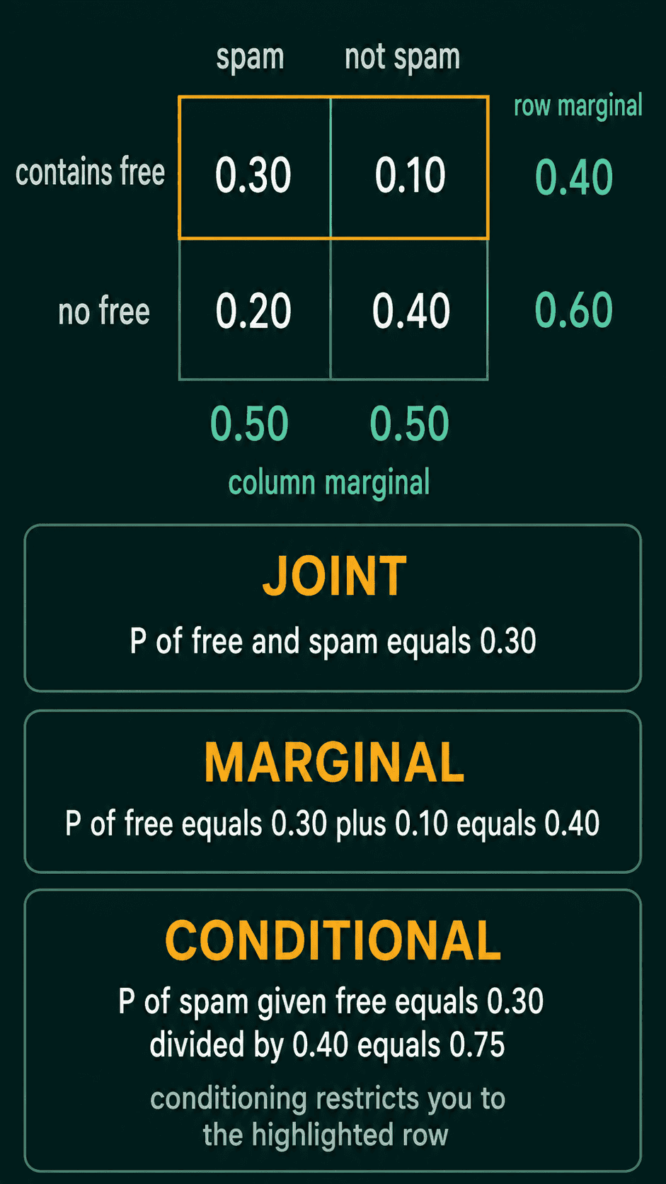
Take two events about an email. $A$ is "the email contains the word free" and $B$ is "the email is spam". Every email lands in one of four cells, and this table gives the probability of each cell:

	spam	not spam
contains free	0.30	0.10
no free	0.20	0.40

The four cells add up to 1, because every email lands in exactly one of them.

The joint probability of $A$ and $B$ is one cell. It is written $P(A, B)$ and read "the probability of $A$ and $B$". The probability that an email contains free and is spam is $P(\text{free}, \text{spam}) = 0.30$.

The marginal probability of $A$ ignores $B$. It is written $P(A)$. To get the probability that an email contains free, add the "contains free" row across both columns: $P(\text{free}) = 0.30 + 0.10 = 0.40$. The name comes from where these totals usually get written, in the margins of the table.

The conditional probability of $B$ given $A$ is the probability of $B$ once you know $A$ happened. It is written $P(B \mid A)$ and read "the probability of $B$ given $A$". Knowing the email contains free means only the top row is possible, and that row holds 0.40 of all emails. Of that 0.40, the spam cell holds 0.30:

$$P(\text{spam} \mid \text{free}) = \frac{0.30}{0.40} = 0.75$$

As a general formula, a conditional probability is the joint probability divided by the marginal probability of the event you condition on:

$$P(B \mid A) = \frac{P(A, B)}{P(A)}$$

Conditioning changes which emails you are looking at. Among all emails, half are spam, since the spam column adds up to $0.30 + 0.20 = 0.50$. Among emails that contain free, 75% are spam.

A spam and free joint table with row and column totals, labelled with the joint 0.30, the marginal 0.40 and the conditional 0.75.

The sum rule and the product rule

Two rules connect the three probabilities.

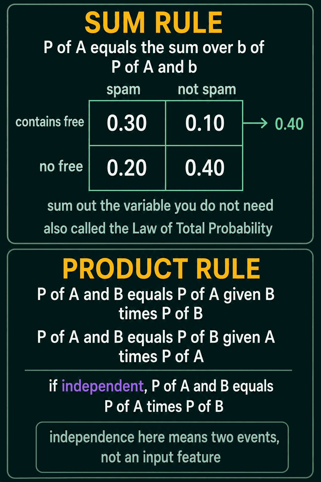
The sum rule gets a marginal from a joint by adding over every value of the variable you no longer care about:

$$P(A) = \sum_b P(A, b)$$

The $\sum_b$ means "add up over every value $b$ that $B$ can take". For $P(\text{free})$, $B$ takes the values spam and not spam. The sum is $0.30 + 0.10 = 0.40$, the same row total as before.

The product rule writes a joint probability as a conditional times a marginal:

$$P(A, B) = P(B \mid A)\,P(A)$$

It works in either direction:

$$P(A, B) = P(A \mid B)\,P(B)$$

Check the first form on the table: $P(\text{spam} \mid \text{free})\,P(\text{free}) = 0.75 \times 0.40 = 0.30$, the joint cell. The product rule adds no new assumption, because it is the conditional probability formula with both sides multiplied by $P(A)$.

Put the two rules together and you get the law of total probability. Split on cases $B_1, \ldots, B_k$ that cannot happen together and between them cover every possibility, such as spam and not spam:

$$P(A) = \sum_i P(A \mid B_i)\,P(B_i)$$

Each term is the product rule, and adding the terms is the sum rule. This is the form to use when you have conditional probabilities and no joint table. Among spam emails, 60% contain free ($0.30 / 0.50$). Among non-spam emails, 20% do ($0.10 / 0.50$), and each group is half of all email:

$$P(\text{free}) = 0.60 \times 0.50 + 0.20 \times 0.50 = 0.40$$

Two events are independent when knowing one tells you nothing about the other, so $P(B \mid A) = P(B)$. The product rule then shortens to:

$$P(A, B) = P(A)\,P(B)$$

The email events are not independent. $P(\text{free})\,P(\text{spam}) = 0.40 \times 0.50 = 0.20$, while the table says $P(\text{free}, \text{spam}) = 0.30$. This "independent" is different from "independent variables" in supervised learning, where it only means the model's inputs.

The sum rule adding the contains free row to 0.40, and the product rule written both ways with its independent special case.

From events to random variables

A random variable is a quantity whose value is uncertain until you observe it, such as the label of an image or the roll of a die. The same three probabilities work for random variables. Instead of two named events, you have a table with one cell for every pair of values.

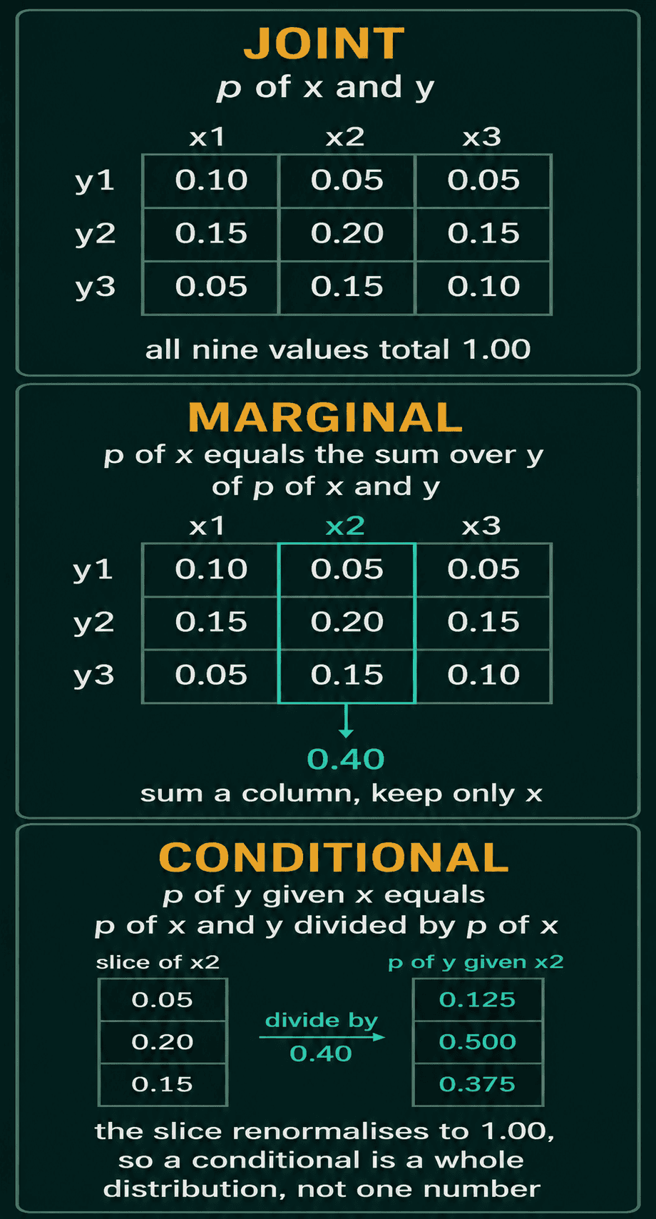
For random variables $X$ and $Y$, the joint distribution $p(x, y)$ gives the probability that $X = x$ and $Y = y$ together. Here $X$ takes the values $x_1, x_2, x_3$ and $Y$ takes $y_1, y_2, y_3$:

$$\begin{array}{c|ccc} & x_1 & x_2 & x_3 \\ \hline y_1 & 0.10 & 0.05 & 0.05 \\ y_2 & 0.15 & 0.20 & 0.15 \\ y_3 & 0.05 & 0.15 & 0.10 \end{array}$$

The marginal distribution of $X$ sums out $Y$, which here means adding down each column:

$$p_X(x) = \sum_y p(x, y)$$

The subscript in $p_X$ says this is the distribution of $X$ alone. Adding down the $x_2$ column gives $p_X(x_2) = 0.05 + 0.20 + 0.15 = 0.40$.

The conditional distribution of $Y$ given $X$ divides by that total:

$$p(y \mid x) = \frac{p(x, y)}{p_X(x)}$$

For $x = x_2$, divide each cell in the $x_2$ column by 0.40. That gives $0.125$ for $y_1$, $0.500$ for $y_2$ and $0.375$ for $y_3$, which add up to 1. A conditional distribution is a whole distribution over every value of $y$, one for each value of $x$ you might condition on, while a conditional probability like $P(\text{spam} \mid \text{free})$ is a single number.

A three by three joint table, the x2 column summed to the marginal 0.40, and that column divided by 0.40 into the conditional distribution 0.125, 0.500 and 0.375.

$p(y \mid x)$ is what many ML models predict. A classifier outputs $p(y \mid x)$, one probability for each label $y$ given the input $x$. A language model outputs $p(\text{next token} \mid \text{previous tokens})$ at every step.

The same ideas carry over to continuous random variables, such as a person's height and weight, with sums replaced by integrals. The joint is then a density $p(x, y)$ over pairs of values, and the marginal comes from integrating out the variable you do not need:

$$p_X(x) = \int p(x, y)\,dy$$

A density is not a probability on its own. A probability comes from integrating the density over a region.

Independence of random variables

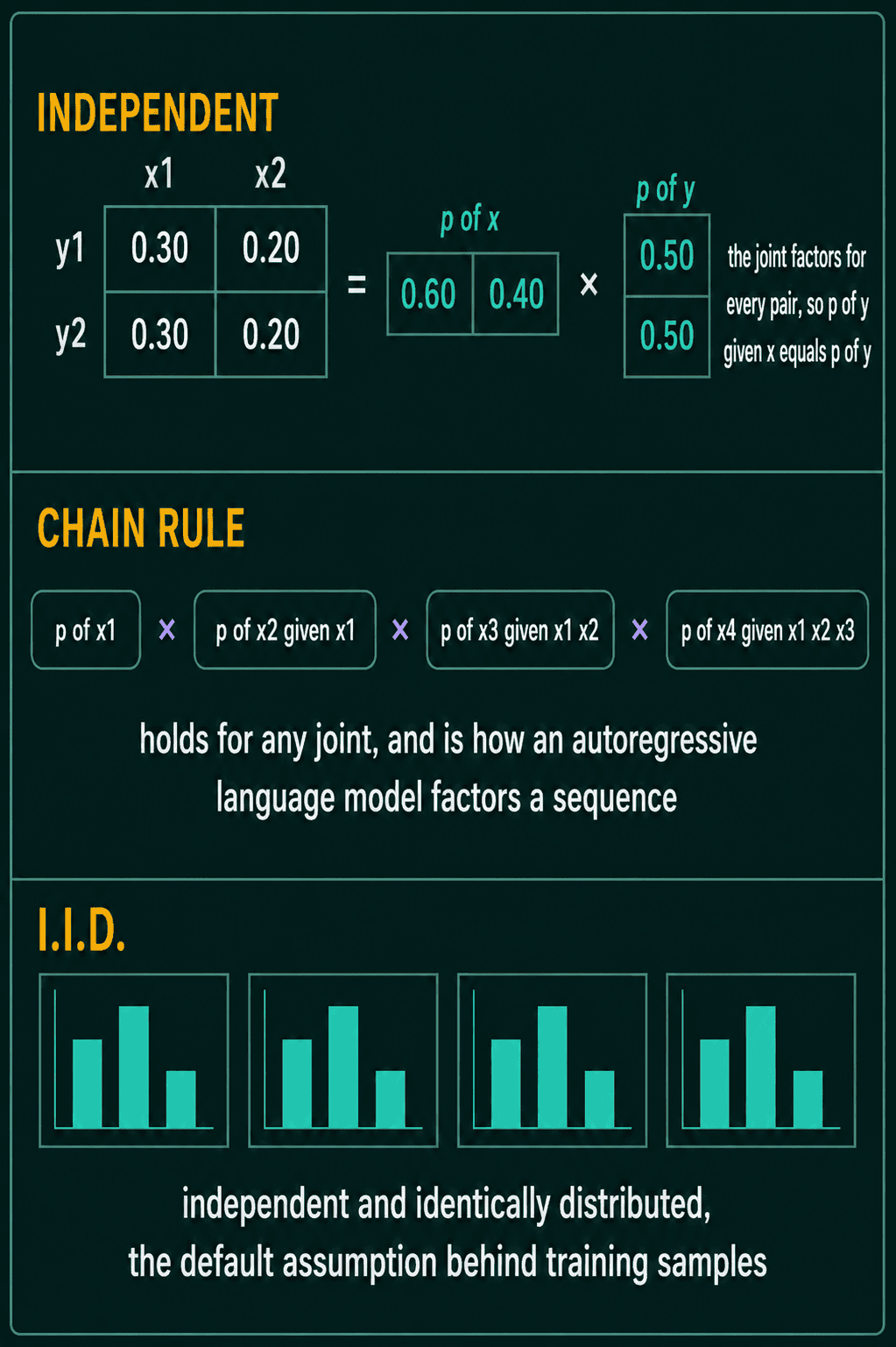
Two random variables are independent if knowing the value of one tells you nothing about the distribution of the other. In terms of the table, the joint is the product of the two marginals in every cell:

$$p(x, y) = p_X(x)\,p_Y(y) \quad \text{for all } x, y$$

It has to hold in every cell, and a match in a few cells is not enough. Here is a table where it does hold:

$$\begin{array}{c|cc} & x_1 & x_2 \\ \hline y_1 & 0.30 & 0.20 \\ y_2 & 0.30 & 0.20 \end{array}$$

The marginals are $p_X = (0.60, 0.40)$ and $p_Y = (0.50, 0.50)$, and every cell equals its column total times its row total: $0.60 \times 0.50 = 0.30$ and $0.40 \times 0.50 = 0.20$. An equivalent test is that conditioning changes nothing. Given $x_1$, the distribution of $Y$ is $0.30 / 0.60 = 0.50$ and $0.30 / 0.60 = 0.50$, the same as $p_Y$:

$$p(y \mid x) = p_Y(y)$$

The three by three table fails the test. Its $p_X(x_2) = 0.40$ and $p_Y(y_2) = 0.50$ multiply to 0.20, which happens to match the $(x_2, y_2)$ cell, while $p_X(x_1)\,p_Y(y_1) = 0.30 \times 0.20 = 0.06$ does not match the 0.10 in the $(x_1, y_1)$ cell.

For many variables, mutual independence means the whole joint is the product of the individual marginals:

$$p(x_1, \ldots, x_n) = p(x_1)\,p(x_2) \cdots p(x_n)$$

Conditional independence and i.i.d.

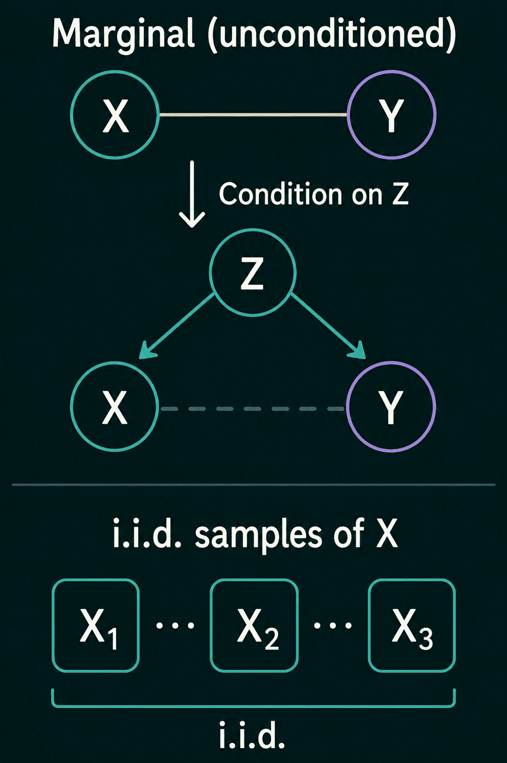
Two variables can be linked across a whole population and stop being linked once you fix a third variable. $X$ and $Y$ are conditionally independent given $Z$, written $X \perp Y \mid Z$, if

$$p(x, y \mid z) = p(x \mid z)\,p(y \mid z) \quad \text{for every } z$$

Take cough and fever as $X$ and $Y$, and whether a person has the flu as $Z$. Across everyone, cough and fever tend to show up together, because the flu makes both more likely. Among people who have the flu, knowing that someone coughs may tell you nothing more about whether they have a fever. Naive Bayes classifiers and hidden Markov models are built on assumptions of this kind.

i.i.d. is short for independent and identically distributed. It describes repeated samples that are mutually independent and all come from the same distribution. A training set is usually treated as i.i.d. samples, and many results about training and evaluation rely on that assumption.

X and Y linked across the population, the link removed after conditioning on Z, and a row of i.i.d. samples of X.

The chain rule of probability

Mutual independence lets you split a joint into a product of marginals, and most variables worth modelling are not independent. The chain rule of probability splits any joint, with no assumptions. Apply the product rule once to peel off the first variable, then again to the rest. For three variables:

$$p(x_1, x_2, x_3) = p(x_1)\,p(x_2 \mid x_1)\,p(x_3 \mid x_1, x_2)$$

Each variable is conditioned on every variable before it. For $n$ variables:

$$p(x_1, \ldots, x_n) = p(x_1)\,p(x_2 \mid x_1) \cdots p(x_n \mid x_1, \ldots, x_{n-1})$$

On the email table, let $x_1$ be the spam label and $x_2$ be whether the email contains free. $p(\text{spam}) = 0.50$ and $p(\text{free} \mid \text{spam}) = 0.30 / 0.50 = 0.60$, so $p(\text{spam}, \text{free}) = 0.50 \times 0.60 = 0.30$, the joint cell from the table. Any ordering of the variables works. Starting from free instead gives $p(\text{free})\,p(\text{spam} \mid \text{free}) = 0.40 \times 0.75 = 0.30$.

Autoregressive language models use this factorization. At each step the model predicts $p(x_n \mid x_1, \ldots, x_{n-1})$, the next token given every token before it. Multiplying those predictions gives the probability of the whole sequence. The tokens of a sentence depend on each other, which is why the chain rule applies and the product of marginals does not.

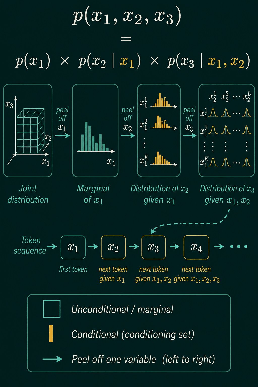
The joint of x1, x2 and x3 factored into the marginal of x1, then x2 given x1, then x3 given x1 and x2, with the same pattern on a token sequence.

When some conditionals simplify, the factorization gets shorter. If $x_3$ stops depending on $x_1$ once $x_2$ is known, then $p(x_3 \mid x_1, x_2) = p(x_3 \mid x_2)$. Graphical models use conditional independence of this kind to keep large joint distributions manageable.

An independent joint table equal to the product of its marginals, the chain rule as a product of conditionals, and i.i.d. samples sharing one distribution.

The same table in PyTorch

A joint distribution of two discrete variables is a 2D tensor, with one row per value of $X$. The sum rule is sum along one axis, and the conditional is a division by the row totals:

1import torch
2 
3# joint[i, j] = p(X = x_i, Y = y_j): one row per value of X
4joint = torch.tensor([
5    [0.10, 0.15, 0.05],   # x1
6    [0.05, 0.20, 0.15],   # x2
7    [0.05, 0.15, 0.10],   # x3
8])
9print(joint.sum())                 # all nine cells
10 
11p_x = joint.sum(dim=1)             # sum rule: add across each row
12p_y = joint.sum(dim=0)             # sum rule: add down each column
13print(p_x, p_y)
14 
15cond = joint / p_x.unsqueeze(1)    # p(y | x): divide each row by its total
16print(cond[1])                     # the distribution of Y given x2
17print(cond.sum(dim=1))             # every row adds up to 1
18# tensor(1.0000)
19# tensor([0.3000, 0.4000, 0.3000]) tensor([0.2000, 0.5000, 0.3000])
20# tensor([0.1250, 0.5000, 0.3750])
21# tensor([1.0000, 1.0000, 1.0000])

The tensor stores the table with $X$ on the rows, so the $x_2$ column of the table above is row 1 here. unsqueeze(1) turns p_x into a column of shape (3, 1), so each row of joint is divided by its own total.

Independence is a cell-by-cell comparison between the joint and the product of its marginals. torch.outer(p_x, p_y) builds that product table:

1import torch
2 
3def is_independent(joint, tol=1e-6):
4    p_x = joint.sum(dim=1)
5    p_y = joint.sum(dim=0)
6    return torch.allclose(joint, torch.outer(p_x, p_y), atol=tol)
7 
8three_by_three = torch.tensor([
9    [0.10, 0.15, 0.05],
10    [0.05, 0.20, 0.15],
11    [0.05, 0.15, 0.10],
12])
13two_by_two = torch.tensor([
14    [0.30, 0.30],   # x1: p(x1, y1), p(x1, y2)
15    [0.20, 0.20],   # x2
16])
17print(is_independent(three_by_three))
18print(is_independent(two_by_two))
19# False
20# True

torch.allclose compares with a small tolerance, because probabilities stored as floats rarely match to the last digit. If a conditional's rows do not add up to 1, check which axis you summed and which axis you divided along.

When to use which, and common mistakes

Use the joint when you need two things at once, the marginal when you only care about one, and the conditional when one value is known and you want the other. Most derivations in probabilistic ML repeat two moves: sum out what you do not need, and split a joint into a conditional times a marginal.

Swapping the conditional. $P(\text{spam} \mid \text{free}) = 0.75$ while $P(\text{free} \mid \text{spam}) = 0.60$. Dividing by the wrong marginal gives the other one.
Multiplying marginals without checking independence. $P(\text{free})\,P(\text{spam})$ gives 0.20 on the email table, and the real joint is 0.30.
Summing or dividing along the wrong axis. In code, dim=0 and dim=1 give different marginals, and a conditional built on the wrong one has rows that do not add up to 1.
Reading "independent variables" as statistical independence. Model inputs are called independent variables even when they are strongly related to each other.

Bayes' theorem uses the product rule written both ways to turn $P(\text{free} \mid \text{spam})$ into $P(\text{spam} \mid \text{free})$. The union bound puts a ceiling on the probability that at least one of several events happens, without knowing their joint. Random variables and their distributions, the PMF for separate values and the PDF for continuous ones, describe a single variable before you put two together.

QuiddityML teaches these ideas as six concepts in the Math track's probability unit, and the exercises on them include writing conditional_from_table and is_independent on a joint tensor and filling in the chain rule factorization for three variables.