By Sagi Shaier · 16 October 2026 · 10 min read
Common probability distributions in ML: Bernoulli, binomial, Poisson, Beta
Which distribution fits which question, the formula and mean of each one worked with real numbers, and how to check them in PyTorch.
A probability distribution says how likely each possible value of a random quantity is, and a handful of named distributions cover most of what machine learning models. A binary classifier's output, the next token a language model picks, the number of requests a server gets in a second and an estimate of a click-through rate each have a distribution that fits them. Knowing which one fits tells you what a model's output means.
Discrete and continuous
A random variable is a quantity whose value comes out of a random process, like the number of heads in 10 coin flips. It is discrete when its values can be counted one by one. Yes or no, a class label and a number of clicks are all discrete. It is continuous when it can take any value on an interval, like a height or a waiting time.
For a discrete variable, each value gets a probability, and the function giving those probabilities is the probability mass function (PMF). $P(X = 3)$ is read "the probability that $X$ equals 3". The probabilities of all the values add up to 1. For a continuous variable, probability comes from the area under a curve called a density, which the second half of this post covers.
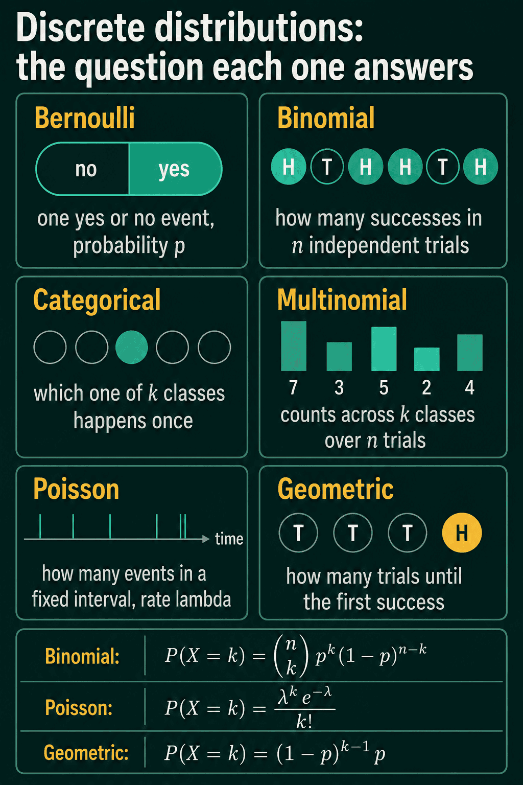
Six discrete distributions and the question each answers
The easiest way to tell the discrete distributions apart is by the question each one answers:
| Distribution | Question it answers |
|---|---|
| Bernoulli | Does one yes/no event happen? |
| Binomial | How many successes in $n$ independent yes/no trials? |
| Categorical | Which one of $k$ classes happens once? |
| Multinomial | How many times does each of $k$ classes happen across $n$ trials? |
| Poisson | How many events happen in a fixed interval? |
| Geometric | How many trials until the first success? |
"Independent" in the binomial row means one trial's outcome does not change the next one's probability.
Two of these show up in most classifiers. Binary classification, like fraud or not fraud, is usually modeled as Bernoulli. Multiclass classification is usually modeled as categorical, and a language model's prediction for the next token is a categorical distribution over its whole vocabulary.
Each distribution has parameters, the numbers that set its shape. Bernoulli has one, $p$, the probability of success. Categorical has a vector $\mathbf{p}$ with one probability per class, and its entries add up to 1.
A class label is usually stored as a vector instead of a single integer. With 4 classes, class 2 (counting from 0) becomes [0, 0, 1, 0], a 1 in the class's position and 0 everywhere else. This is called 1-of-K encoding or one-hot encoding, and it is the format a classifier's predicted probability vector gets compared against when the loss is computed.
Bernoulli: one yes/no trial
A Bernoulli variable is a single trial that comes out 1 (success) with probability $p$ and 0 (failure) with probability $1-p$. Its PMF packs both cases into one formula:
$$P(X=x) = p^{x}(1-p)^{1-x}, \quad x \in \{0, 1\}$$
The exponents pick the right case. With $p = 0.3$, setting $x = 1$ gives $0.3^1 \times 0.7^0 = 0.3$, and setting $x = 0$ gives $0.3^0 \times 0.7^1 = 0.7$.
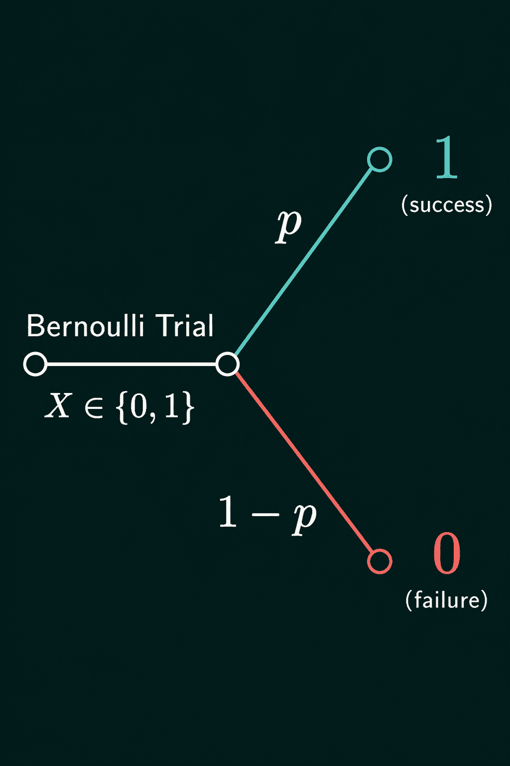
The mean $E[X]$ is the average value over many trials, and the variance $\text{Var}(X)$ measures how spread out the values are around that mean:
$$E[X] = p \qquad \text{Var}(X) = p(1-p)$$
At $p = 0.3$ the mean is 0.3 and the variance is $0.3 \times 0.7 = 0.21$. The variance is largest at $p = 0.5$, where it is $0.25$ and the outcome is hardest to predict. It drops to 0 at $p = 0$ and $p = 1$, where the outcome is fixed.
Binomial: counting successes in n trials
Run $n$ independent Bernoulli trials with the same $p$ and count the successes. That count $K$ follows a binomial distribution, written $K \sim \text{Bin}(n, p)$, read "$K$ is binomial with parameters $n$ and $p$". Its PMF is:
$$P(K=k) = \binom{n}{k}p^{k}(1-p)^{n-k}$$
There are three pieces. $p^{k}$ is the probability of the $k$ successes, $(1-p)^{n-k}$ is the probability of the $n-k$ failures, and $\binom{n}{k}$, read "$n$ choose $k$", counts how many different orders of successes and failures give the same total.
A worked example: 10 people get an email, and each opens it with probability 0.3. The probability that exactly 3 open it is:
$$\binom{10}{3} \times 0.3^{3} \times 0.7^{7} = 120 \times 0.027 \times 0.0824 = 0.267$$
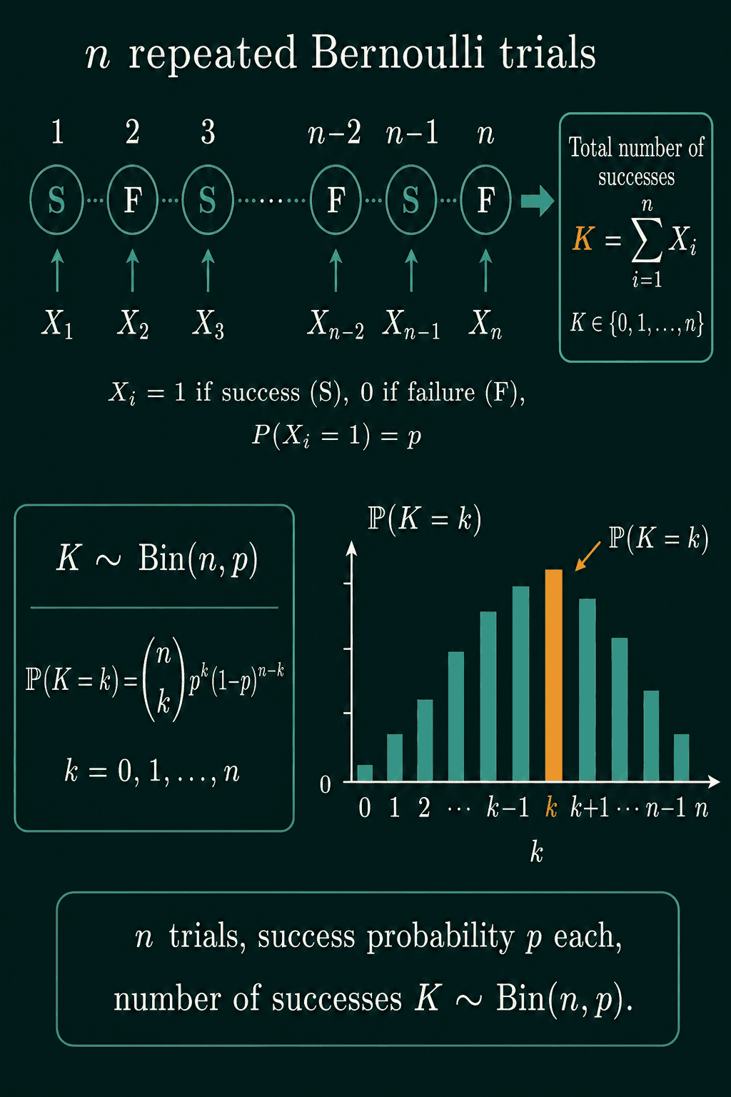
Because a binomial is $n$ independent Bernoulli trials added together, its mean and variance are $n$ times one trial's:
$$E[K] = np \qquad \text{Var}(K) = np(1-p)$$
For the email example, the mean is $10 \times 0.3 = 3$ opens and the variance is $10 \times 0.3 \times 0.7 = 2.1$. These two formulas are a fast sanity check on any "how many out of $n$" number. A model that predicts 9 opens out of 10 for a group with an open rate of 0.3 is far from the mean of 3.
Poisson: counting events in a fixed window
The Poisson distribution counts how many events land in a fixed window of time or space, when the events happen independently at an average rate $\lambda$ (lambda) per window. Requests to a server per second, typos per page and photons hitting a camera sensor per exposure are all Poisson-style counts. Its PMF is:
$$P(X=k) = \frac{\lambda^{k}e^{-\lambda}}{k!}$$
Here $e \approx 2.718$ and $k!$ is $k \times (k-1) \times \dots \times 1$. A binomial has a fixed number of trials $n$, so it can never count more than $n$ successes. A Poisson has no such cap, only an average rate.
With $\lambda = 5$ requests per second, the probability of exactly 9 requests in the next second is $5^{9} e^{-5} / 9! = 0.036$.
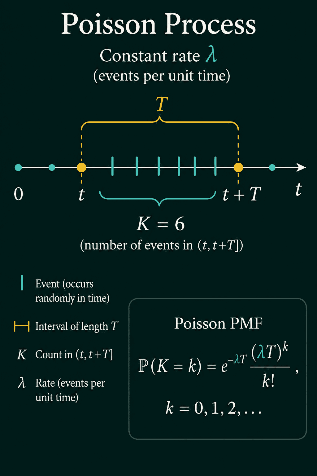
The picture writes the rate per unit of time, so a window of length $T$ has an average of $\lambda T$ events, and $\lambda T$ takes the place of $\lambda$ in the formula. With a window of length 1, the two are the same.
The Poisson's one parameter is both its mean and its variance:
$$E[X] = \lambda \qquad \text{Var}(X) = \lambda$$
At 5 requests per second, the average is 5 and the standard deviation (the square root of the variance) is $\sqrt{5} \approx 2.24$. A second with 9 requests is normal for this rate. A second with 40 has a probability of about $7.5 \times 10^{-23}$, so it means something other than steady traffic is going on.
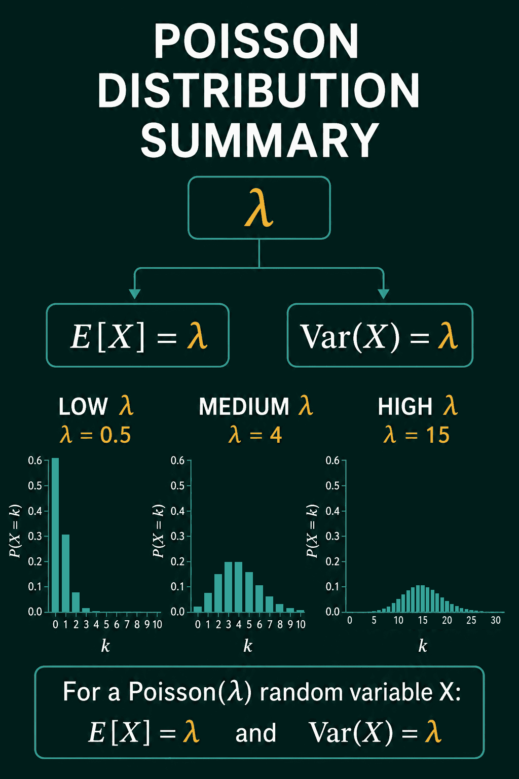
That equality is also a test. If count data has a sample variance far above its sample mean, it is called overdispersed, and no choice of $\lambda$ will make a Poisson fit it.
The discrete distributions on one page
The geometric distribution from the table also has a short PMF. The first success landing on trial $k$ means $k-1$ failures and then one success, so $P(X = k) = (1-p)^{k-1}p$.
Continuous distributions
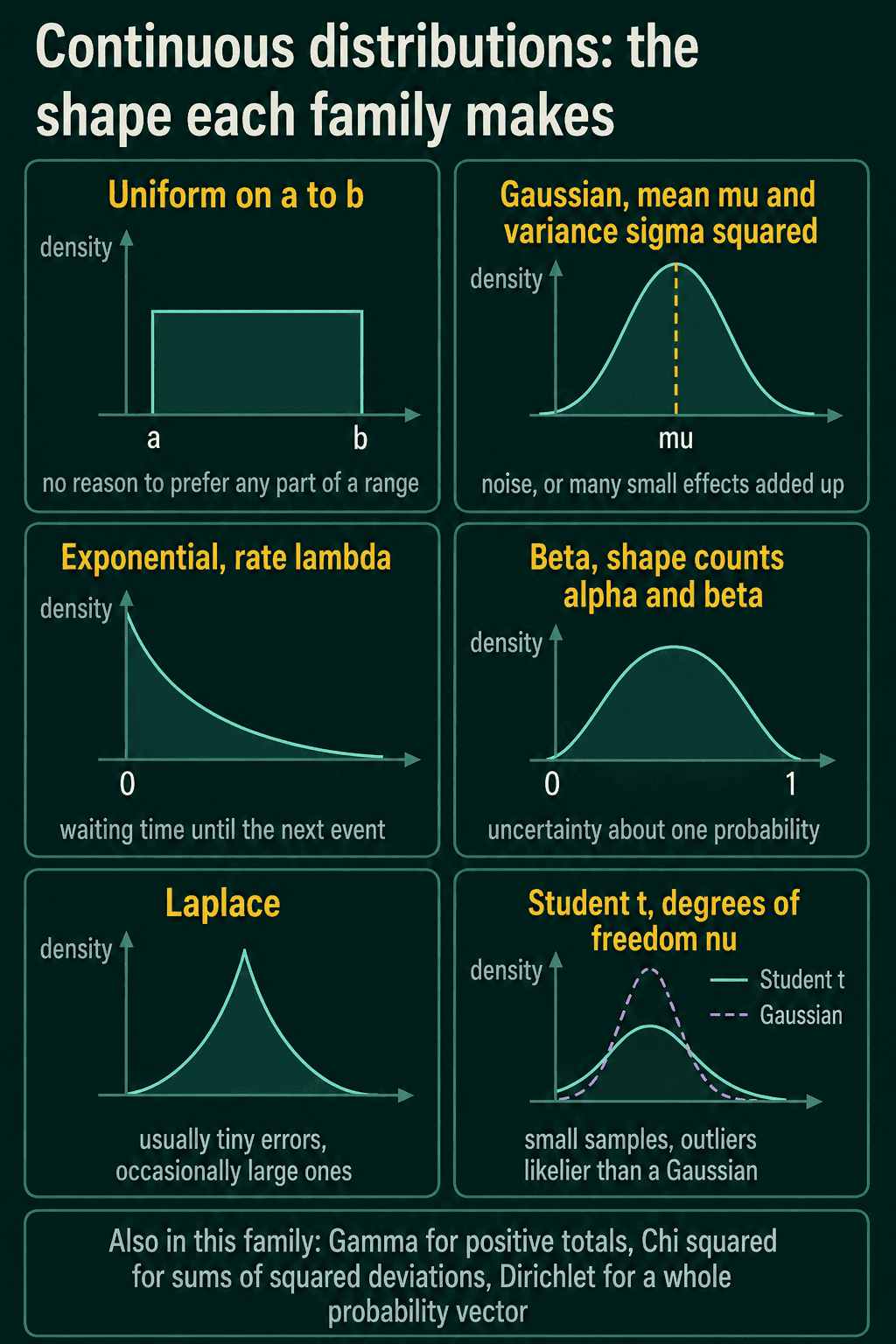
Continuous distributions describe quantities on an interval or the whole number line: height, time, sensor noise, a regression error. The probability of landing in a range is the area under the density curve over that range. These five families show up often:
- Uniform: every value in an interval $[a, b]$ has the same density.
- Gaussian (normal): the bell curve, set by a mean and a variance.
- Exponential: the waiting time until the next event when events arrive at a Poisson rate $\lambda$.
- Laplace: a sharper peak and heavier tails than a Gaussian, so values far from the center are more likely. It is connected to absolute error.
- Student's t: a Gaussian-like center with heavier tails, set by a number called its degrees of freedom $\nu$ (nu).
What separates them is what each assumes about the values: which values are allowed, whether the shape is symmetric, and how quickly the tails fall off.
Support: which values a distribution allows
The set of values a distribution can produce is its support. Some continuous distributions are restricted to part of the number line:
- Beta lives on $[0, 1]$, so it fits probabilities and proportions.
- Gamma and chi-squared live on values of 0 and up, so they fit waiting times, scales and sums of squared Gaussian values.
- Dirichlet lives on probability vectors, whose entries are 0 or more and add up to 1. It is the version of Beta for a whole vector of probabilities.
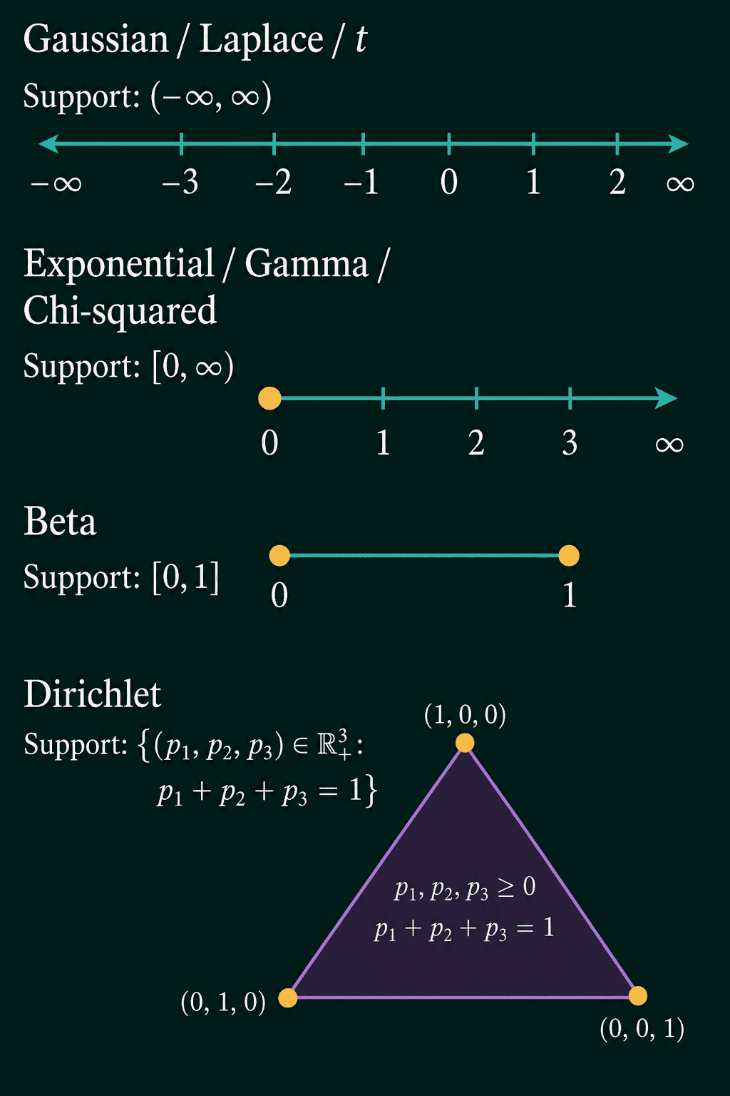
The support is a quick check on a modeling choice. A Gaussian puts some probability on negative values, so it is a poor default for a quantity that cannot go below zero, like a duration. A Beta cannot leave $[0, 1]$, so it is a good default for uncertainty about a probability.
Beta: a distribution over a probability
Most distributions describe data. Beta describes a probability you are still estimating, like the click-through rate of an ad after a few hundred impressions. Its density has two shape parameters, $\alpha$ (alpha) and $\beta$ (beta):
$$p(x) \propto x^{\alpha-1}(1-x)^{\beta-1}, \quad 0 \le x \le 1$$
The $\propto$ means "proportional to". It hides a constant that makes the total area 1, and the shape comes entirely from the two exponents. The mean is:
$$E[X] = \frac{\alpha}{\alpha+\beta}$$
Beta(8, 4) has a mean of $8 / 12 \approx 0.67$. Beta(1, 1) has both exponents equal to 0, so $p(x) \propto 1$, the flat uniform distribution on $[0, 1]$.
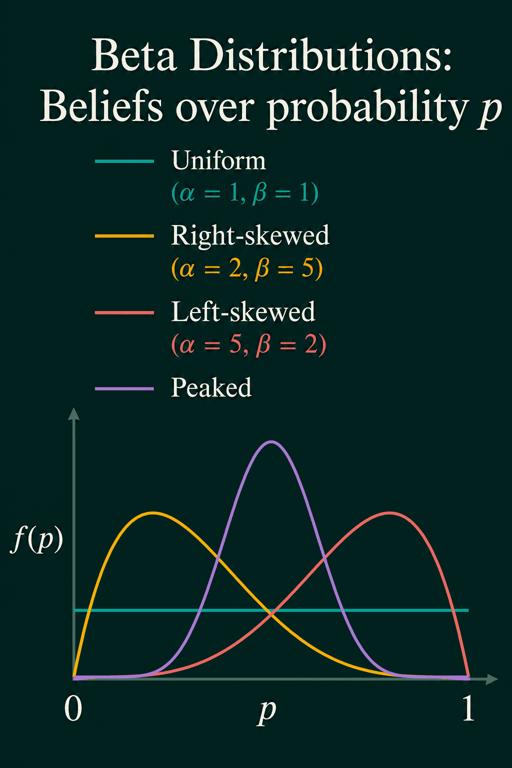
Larger $\alpha + \beta$ gives a narrower curve. Beta(10, 10) and Beta(1, 1) both have a mean of 0.5, and Beta(10, 10) is far more concentrated around it.
Alpha and beta as pseudo-counts
$\alpha$ and $\beta$ behave like counts of successes and failures the distribution has already seen, so they are called pseudo-counts. The mean $\alpha / (\alpha + \beta)$ is the success rate of those imaginary trials. When a Beta is the starting belief before any real data, it is called a prior, and its mean is the expected success rate before you look at the data.
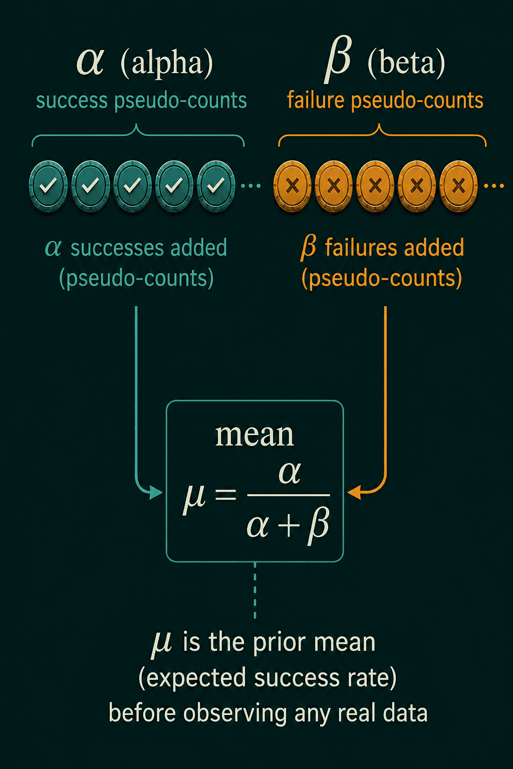
Strictly, the density has the same shape as the probability of $\alpha - 1$ successes and $\beta - 1$ failures, so Beta(8, 4) carries about as much weight as 7 successes and 3 failures already observed. Each real success adds 1 to $\alpha$ and each real failure adds 1 to $\beta$. One more click turns Beta(8, 4) into Beta(9, 4), and the mean moves from $8/12 \approx 0.667$ to $9/13 \approx 0.692$. That update is why Beta pairs so well with Bernoulli data.
Checking the numbers in PyTorch
torch.distributions has every distribution in this post. log_prob returns the log of the probability, and .exp() turns it back into a probability:
1import torch
2from torch.distributions import Bernoulli, Binomial, Poisson, Beta
3
4coin = Bernoulli(probs=torch.tensor(0.3))
5print(coin.log_prob(torch.tensor([0.0, 1.0])).exp())  # P(X=0), P(X=1)
6print(coin.mean, coin.variance)
7
8opens = Binomial(total_count=10, probs=torch.tensor(0.3))
9print(opens.log_prob(torch.tensor(3.0)).exp())        # P(K=3)
10print(opens.mean, opens.variance)
11
12requests = Poisson(rate=torch.tensor(5.0))
13print(requests.log_prob(torch.tensor([5.0, 9.0, 40.0])).exp())
14print(requests.mean, requests.variance)
15
16ctr = Beta(torch.tensor(8.0), torch.tensor(4.0))
17print(ctr.mean)
18# tensor([0.7000, 0.3000])
19# tensor(0.3000) tensor(0.2100)
20# tensor(0.2668)
21# tensor(3.) tensor(2.1000)
22# tensor([1.7547e-01, 3.6266e-02, 7.5107e-23])
23# tensor(5.) tensor(5.)
24# tensor(0.6667)
Every number matches the hand calculations above. The overdispersion test takes a few more lines. Steady traffic at 5 requests per second gives a sample mean and variance that agree. Traffic where 80% of seconds are quiet (rate 1) and 20% are busy (rate 20) has about the same mean and a much larger variance:
1import torch
2from torch.distributions import Poisson
3
4torch.manual_seed(0)
5steady = Poisson(torch.tensor(5.0)).sample((10_000,))
6print(round(steady.mean().item(), 2), round(steady.var().item(), 2))
7
8# bursty traffic: each second is either quiet (rate 1) or busy (rate 20)
9rates = torch.where(torch.rand(10_000) < 0.8, 1.0, 20.0)
10bursty = Poisson(rates).sample()
11print(round(bursty.mean().item(), 2), round(bursty.var().item(), 2))
12# 5.0 5.0
13# 4.77 61.63
A variance of 61.63 next to a mean of 4.77 means a single Poisson is the wrong model for the bursty counts. If log_prob raises a ValueError on a binomial or Poisson, check that the value is a whole number inside the support. 3.0 works, while 3.5, -1.0 or 11 successes out of total_count=10 raise the error.
Picking a distribution, and common mistakes
Start from the question the data answers. One yes/no outcome is Bernoulli and one class out of many is categorical. A count of successes out of a fixed $n$ is binomial, and a count with no fixed cap is Poisson. A quantity that is itself a probability is Beta.
- Using a binomial without a fixed $n$. Requests per second have no maximum number of trials, so they are Poisson counts.
- Fitting a Poisson to overdispersed counts. Compare the sample mean and variance first. Bursty data like the example above breaks the Poisson's mean-equals-variance rule.
- Ignoring the support. A Gaussian for a duration or a price puts probability on negative values. A Beta for a probability stays in $[0, 1]$.
- Mixing up the Beta pseudo-counts. The mean uses $\alpha$ and $\beta$ directly, $8 / 12$ for Beta(8, 4). The "already observed" counts are $\alpha - 1$ and $\beta - 1$.
Related concepts
Random variables and the PMF vs PDF distinction are the base this post builds on. The Gaussian distribution is the continuous distribution ML uses most, with its own formula, standardization and log-density. Degrees of freedom is the parameter behind Student's t and chi-squared. Bayes' theorem is the rule behind the Beta update, where a prior is combined with data to give an updated belief called the posterior.
QuiddityML teaches these distributions as five concepts in the Math track's probability unit, and the exercises include filling in the binomial probability of 2 heads in 4 fair flips, writing binomial_moments from scratch and working out the Beta shape counts after 7 successes and 3 failures.