By Sagi Shaier · 16 October 2026 · 5 min read
Degrees of freedom explained
Why sample variance divides by n - 1, what the degrees of freedom of Student's t and chi-squared control, and a PyTorch simulation that shows dividing by n runs low.
Degrees of freedom is the number of values that are still free to vary once the constraints on them are fixed. The count comes up whenever a statistic is computed from data that was already used to estimate something else, like a mean.
Three numbers with a fixed average
Say three numbers must have an average of 10, so they must add up to 30. You can pick the first two freely. If you choose 12 and 7, the third number has no choice left: it must be $30 - 12 - 7 = 11$.
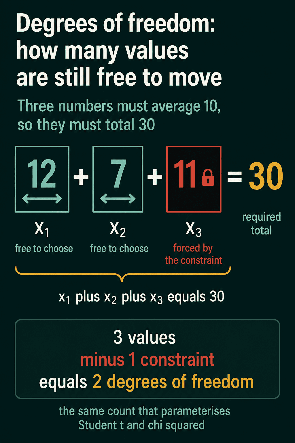
There are 3 values and 1 constraint, the fixed total, so there are 2 degrees of freedom. In general, each constraint the values must satisfy removes one degree of freedom.
Sample variance and the n - 1
The same counting explains a common place degrees of freedom show up. You have $n$ measurements $x_1, \dots, x_n$. Their sample mean $\bar{x}$ (read "x bar") is their average:
$$\bar{x} = \frac{1}{n}\sum_{i=1}^{n} x_i$$
The $\sum_{i=1}^{n}$ means "add up the terms for $i = 1$ to $n$". The usual estimate of how spread out the measurements are is the sample variance:
$$s^2 = \frac{1}{n-1}\sum_{i=1}^{n} (x_i-\bar{x})^2$$
Each $x_i - \bar{x}$ is a deviation, how far one measurement sits from the mean. The sample variance adds up the squared deviations and divides by $n - 1$.
The $n - 1$ is a degrees-of-freedom count. The deviations always add up to exactly 0, because $\bar{x}$ was computed from the same $n$ numbers. Take the measurements 4, 7 and 13. Their mean is 8, and their deviations are $-4$, $-1$ and $5$, which add up to 0. Once you know any two of the deviations, the third is forced, the same way the third number was forced above. There are $n$ deviations but only $n - 1$ of them are free, so the sum of squares is divided by $n - 1$:
$$s^2 = \frac{(-4)^2 + (-1)^2 + 5^2}{3 - 1} = \frac{42}{2} = 21$$
Dividing by $n = 3$ instead gives 14.
Why dividing by n runs low
Dividing by $n$ when the mean came from the same data gives estimates that are too small on average. An estimator whose average is off from the true value in one direction is called biased, and this one is biased downward. The deviations are measured from $\bar{x}$, which sits in the middle of this particular sample, so they come out smaller than deviations from the true mean would. Dividing by $n - 1$ makes up for that. Estimating a quantity from data uses up one degree of freedom for each quantity it has to estimate first, here the mean.
If the true mean were known ahead of time and not estimated from the sample, nothing would constrain the deviations, and dividing by $n$ would be right.
Degrees of freedom in Student's t and chi-squared
Two distributions take degrees of freedom as their parameter, usually written $\nu$ (nu). The chi-squared distribution with $\nu$ degrees of freedom is the distribution of a sum of $\nu$ squared standard Gaussian values, so it only takes values of 0 and up. Student's t has a bell shape like a Gaussian with heavier tails, which means values far from the center are more likely.
More degrees of freedom means more independent information went into the statistic. As $\nu$ grows, Student's t gets closer and closer to a standard Gaussian. At $\nu = 1$ its tails are far heavier, and by $\nu = 30$ it is hard to tell the two apart near the center.
Degrees of freedom in PyTorch
The deviations add up to 0, and torch.var takes a correction argument that picks the divisor, $n$ minus correction:
1import torch
2
3x = torch.tensor([4.0, 7.0, 13.0])
4dev = x - x.mean()
5print(dev, dev.sum())
6print(x.var(correction=0), x.var(correction=1))
7# tensor([-4., -1.,  5.]) tensor(0.)
8# tensor(14.) tensor(21.)
correction=0 divides by $n$ and correction=1 divides by $n - 1$, the default. The bias shows up in a simulation. Draw 100,000 samples of 5 values each from a Gaussian with standard deviation 2, so the true variance is 4, and average each estimator across the samples:
1import torch
2
3torch.manual_seed(0)
4samples = torch.randn(100_000, 5) * 2.0   # 100,000 samples of n = 5, true variance 4
5
6divide_by_n = samples.var(dim=1, correction=0).mean()
7divide_by_n_minus_1 = samples.var(dim=1, correction=1).mean()
8print(round(divide_by_n.item(), 2), round(divide_by_n_minus_1.item(), 2))
9# 3.21 4.01
Dividing by $n$ averages 3.21, about $4 \times 4/5$. Dividing by $n - 1$ averages 4.01, close to the true 4. With $n = 5$ the gap is 20%, and it shrinks as $n$ grows.
Student's t approaching a Gaussian is visible in the density values at the center, $x = 0$, and out in the tail, $x = 3$:
1import torch
2from torch.distributions import StudentT, Normal
3
4points = torch.tensor([0.0, 3.0])
5for df in [1.0, 5.0, 30.0]:
6    print(df, StudentT(df).log_prob(points).exp())
7print("normal", Normal(0.0, 1.0).log_prob(points).exp())
8# 1.0 tensor([0.3183, 0.0318])
9# 5.0 tensor([0.3796, 0.0173])
10# 30.0 tensor([0.3956, 0.0068])
11# normal tensor([0.3989, 0.0044])
At $\nu = 1$ the density at 3 is 0.0318, about 7 times the Gaussian's 0.0044. At $\nu = 30$ the center is 0.3956 against the Gaussian's 0.3989.
When the correction counts, and common mistakes
The difference between $n$ and $n - 1$ is large for small samples and small for big ones. With 5 values it is 20%, and with 1000 values it is 0.1%. It counts most when you estimate spread from a handful of runs, like the variance of a metric across 5 random seeds.
- Mixing up library defaults.
torch.varandtorch.stddivide by $n - 1$ by default. NumPy'snp.varandnp.stddivide by $n$ by default (ddof=0). The same data gives two different answers across the two libraries. - Using $n - 1$ when the mean is known. If the mean was fixed ahead of time and not computed from the sample, divide by $n$.
- Reading degrees of freedom as the sample size. It is the sample size minus the number of quantities estimated from it.
Related concepts
Common probability distributions places Student's t and chi-squared among the other continuous families. The Gaussian distribution is what Student's t approaches as $\nu$ grows. Expected value and variance define the variance that $s^2$ estimates. In ML, the phrase also shows up more loosely for model complexity or the effective number of parameters, with the same question behind it: how many independent pieces can actually move?
QuiddityML teaches degrees of freedom as a concept in the Math track's probability unit, and the exercises on it include counting how many values are still free when three numbers must add to 30.