By Sagi Shaier · 17 October 2026 · 8 min read
Expected value and variance explained, with conditional expectation
How to compute the expected value and variance of a distribution by hand and in PyTorch, what happens to them when you shift or scale the data, and why a model trained with squared error predicts a conditional mean.
The expected value of a random quantity is its probability-weighted average, the value it comes out at on average. The variance measures how far it typically lands from that average. A whole distribution has a lot of detail, and these two numbers summarize where it sits and how spread out it is. They are also the language of ML: a training loss is an average over data, and noise, uncertainty and unstable estimates are all described with variance.
A running example
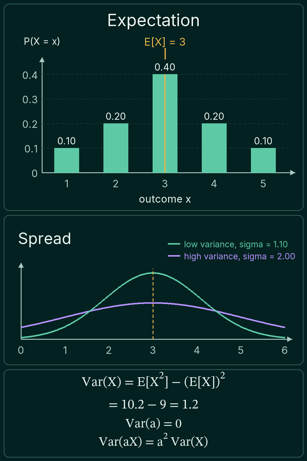
A random variable is a quantity whose value comes out of a random process. It is written with a capital letter like $X$. Take a variable $X$ that can be 1, 2, 3, 4 or 5, with these probabilities:
| Value $x$ | Probability $P(X = x)$ |
|---|---|
| 1 | 0.1 |
| 2 | 0.2 |
| 3 | 0.4 |
| 4 | 0.2 |
| 5 | 0.1 |
The probabilities add up to 1, and the distribution is symmetric around 3.
The expected value
The expected value of $X$ is written $\mathbb{E}[X]$. Multiply each value by its probability and add the products:
$$\mathbb{E}[X] = \sum_x x\,P(X=x)$$
For the example:
$$\mathbb{E}[X] = 1(0.1) + 2(0.2) + 3(0.4)$$
$$+ 4(0.2) + 5(0.1) = 3$$
Values with more probability pull the average toward themselves. A plain average of the five values would also be 3 here, but only because the probabilities are symmetric. Change $P(X=5)$ to 0.3 and $P(X=3)$ to 0.2, and the expected value moves up to 3.4.
The expected value is also called the expectation or the mean of the distribution, and it is often written $\mu$ (mu). It does not have to be a value $X$ can take. A fair coin scored 0 or 1 has an expected value of 0.5.
Expectation is linear
Expectation has a property that makes it easy to work with. For any numbers $a$ and $b$ and any two random variables $X$ and $Y$:
$$\mathbb{E}[aX + bY] = a\,\mathbb{E}[X] + b\,\mathbb{E}[Y]$$
This holds whether or not $X$ and $Y$ depend on each other. For example, $\mathbb{E}[X + X] = 6$, even though the two copies of $X$ are as dependent as two quantities can be. A constant also passes straight through, so $\mathbb{E}[2X + 5] = 2 \times 3 + 5 = 11$.
Linearity is why expected losses are easy to handle. The expected loss over a dataset is the average of the expected losses of the individual examples, and you can compute or estimate each piece on its own.
The variance
Two distributions can have the same expected value and very different spread. The variance measures the spread as the expected squared distance from the mean:
$$\mathrm{Var}(X) = \mathbb{E}\big[(X - \mathbb{E}[X])^2\big]$$
For the example, the squared distances from 3 are 4, 1, 0, 1 and 4. Weighting them by the probabilities gives
$$\mathrm{Var}(X) = 4(0.1) + 1(0.2) + 0(0.4)$$
$$+ 1(0.2) + 4(0.1) = 1.2$$
The distance is squared so that points below the mean and above it both add to the spread, rather than cancelling. The cost is the units. If $X$ is in meters, the variance is in square meters. The standard deviation $\sigma$ (sigma) is the square root of the variance, back in the original units. Here $\sigma = \sqrt{1.2} = 1.10$.
There is a second way to compute the same number, which is often easier in code:
$$\mathrm{Var}(X) = \mathbb{E}[X^2] - (\mathbb{E}[X])^2$$
$\mathbb{E}[X^2]$ is the expected value of $X$ squared: $1(0.1) + 4(0.2) + 9(0.4) + 16(0.2) + 25(0.1) = 10.2$. Subtracting $3^2 = 9$ gives 1.2 again.
Shifting and scaling
Adding a constant $b$ to $X$ moves every value by the same amount, so the mean moves and the spread does not. Multiplying $X$ by $a$ multiplies every distance from the mean by $a$, so every squared distance is multiplied by $a^2$:
$$\mathrm{Var}(aX + b) = a^2\,\mathrm{Var}(X)$$
So $\mathrm{Var}(2X + 5) = 4 \times 1.2 = 4.8$, and the standard deviation doubles from 1.10 to 2.19. A constant on its own has no spread, so $\mathrm{Var}(b) = 0$.
Mean and variance in PyTorch
With the values in one tensor and their probabilities in another, (values * probs).sum() is the expected value. It multiplies each value by its probability and adds the products. The variance is the same pattern applied to the squared distances:
1import torch
2
3values = torch.tensor([1.0, 2.0, 3.0, 4.0, 5.0])
4probs = torch.tensor([0.1, 0.2, 0.4, 0.2, 0.1])
5
6def mean_and_variance(values, probs):
7    mean = (values * probs).sum()
8    var = ((values - mean) ** 2 * probs).sum()
9    return mean, var
10
11mean, var = mean_and_variance(values, probs)
12second_moment = (values ** 2 * probs).sum()
13print(mean, var, var.sqrt())
14print(second_moment, second_moment - mean ** 2)
15print(mean_and_variance(2 * values + 5, probs))
16# tensor(3.) tensor(1.2000) tensor(1.0954)
17# tensor(10.2000) tensor(1.2000)
18# (tensor(11.), tensor(4.8000))
The last line checks the shift and scale rules: $2X + 5$ has mean 11 and variance 4.8.
The expected value is what a long-run average of samples settles toward. Draw 100,000 values from the distribution and their plain average and variance come out close to 3 and 1.2:
1import torch
2
3torch.manual_seed(0)
4x = torch.multinomial(torch.tensor([0.1, 0.2, 0.4, 0.2, 0.1]), 100_000, replacement=True).float() + 1
5print(x.mean(), x.var(correction=0))
6# tensor(3.0015) tensor(1.2018)
Continuous variables and moments
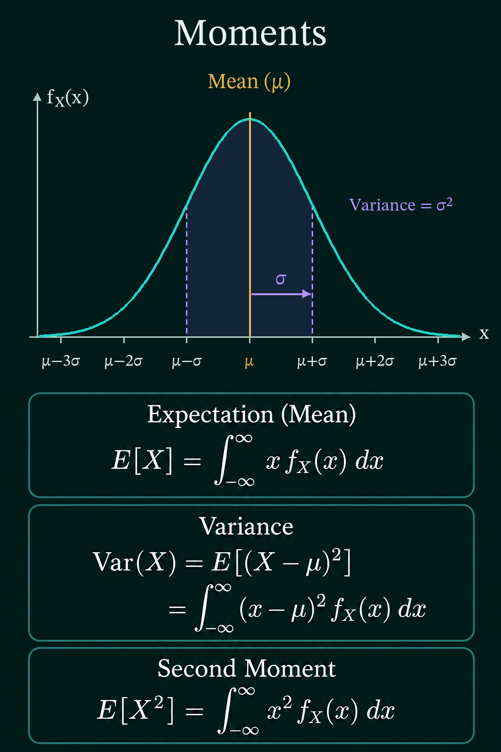
For a continuous variable with density $f_X(x)$, the sum becomes an integral, which adds up $x$ times the density over every value:
$$\mathbb{E}[X] = \int_{-\infty}^{\infty} x\,f_X(x)\,dx$$
The variance and $\mathbb{E}[X^2]$ follow the same pattern, with $(x - \mu)^2$ or $x^2$ in place of $x$.
These are examples of moments, expectations of powers of a random variable. The first moment $\mathbb{E}[X]$ is the mean. The second moment $\mathbb{E}[X^2]$, together with the mean, gives the variance. Higher moments, built from the third and fourth powers, describe the shape further: whether the distribution leans to one side and how heavy its tails are.
Conditional expectation
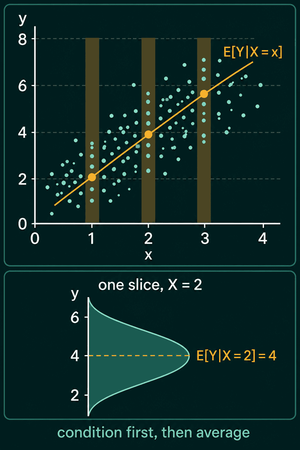
Often you know something about the situation, and you want the average given that information. A conditional expectation is the expected value of $Y$ after you learn that $X = x$:
$$\mathbb{E}[Y \mid X=x] = \sum_y y\,P(Y=y \mid X=x)$$
The vertical bar reads "given". $P(Y = y \mid X = x)$ is the probability that $Y = y$ among only the cases where $X = x$. So the formula keeps only the cases where $X = x$, then averages $Y$ inside that slice. For a continuous $Y$ the sum becomes an integral, $\int y\,p(y \mid x)\,dy$.
For a worked example, let $X$ be 0 or 1 with equal probability, and $Y$ be 0, 1 or 2. The joint probability $P(X = x, Y = y)$ is the probability that both happen at once. When $X = 0$ the joint probabilities of $Y = 0, 1, 2$ are 0.30, 0.15 and 0.05. When $X = 1$ they are 0.05, 0.15 and 0.30. Each row adds up to 0.5, which is $P(X = x)$. Dividing a row by 0.5 gives the conditional probabilities inside that slice: 0.6, 0.3 and 0.1 when $X = 0$. Then
$$\mathbb{E}[Y \mid X=0] = 0(0.6) + 1(0.3) + 2(0.1) = 0.5$$
and the same steps on the second row give $\mathbb{E}[Y \mid X=1] = 1.5$.
The law of total expectation
$\mathbb{E}[Y \mid X]$ is itself a random variable, because its value depends on which $X$ comes out. Here it is 0.5 half the time and 1.5 the other half. Taking its expected value returns the plain expected value of $Y$:
$$\mathbb{E}\big[\mathbb{E}[Y \mid X]\big] = \mathbb{E}[Y]$$
This is the law of total expectation. In the example, $0.5(0.5) + 0.5(1.5) = 1$. Computing $\mathbb{E}[Y]$ directly gives the same answer: adding the columns, $Y$ is 0, 1 and 2 with probabilities 0.35, 0.30 and 0.35, and the expected value is 1. The law lets you compute a hard expectation by splitting it into easier conditional pieces and averaging the pieces.
Variance splits in a similar way:
$$\mathrm{Var}(Y) = \mathbb{E}\big[\mathrm{Var}(Y\mid X)\big] + \mathrm{Var}\big(\mathbb{E}[Y\mid X]\big)$$
The first term is the average spread inside each slice. The second is how much the slice averages differ from each other. In code:
1import torch
2
3y_values = torch.tensor([0.0, 1.0, 2.0])
4# rows: X = 0, X = 1. columns: Y = 0, 1, 2
5joint = torch.tensor([[0.30, 0.15, 0.05],
6                      [0.05, 0.15, 0.30]])
7
8p_x = joint.sum(dim=1)                    # P(X = x)
9p_y_given_x = joint / p_x[:, None]        # each row now sums to 1
10cond_mean = (p_y_given_x * y_values).sum(dim=1)
11print(p_x, cond_mean)
12
13print((p_x * cond_mean).sum())            # E[E[Y | X]]
14print((joint.sum(dim=0) * y_values).sum())  # E[Y] from the marginal of Y
15# tensor([0.5000, 0.5000]) tensor([0.5000, 1.5000])
16# tensor(1.)
17# tensor(1.)1import torch
2
3y_values = torch.tensor([0.0, 1.0, 2.0])
4joint = torch.tensor([[0.30, 0.15, 0.05],
5 [0.05, 0.15, 0.30]])
6p_x = joint.sum(dim=1)
7p_y_given_x = joint / p_x[:, None]
8
9cond_mean = (p_y_given_x * y_values).sum(dim=1)
10cond_var = (p_y_given_x * (y_values - cond_mean[:, None]) ** 2).sum(dim=1)
11
12within = (p_x * cond_var).sum() # E[Var(Y | X)]
13between = (p_x * (cond_mean - 1.0) ** 2).sum() # Var(E[Y | X]), E[Y] = 1
14p_y = joint.sum(dim=0)
15total = (p_y * (y_values - 1.0) ** 2).sum() # Var(Y)
16print(cond_var, within, between, total)
17# tensor([0.4500, 0.4500]) tensor(0.4500) tensor(0.2500) tensor(0.7000)The spread inside the slices (0.45) plus the spread between the slice averages (0.25) adds up to the total variance of 0.7.
Why regression predicts a conditional mean
A regression model predicts a number $Y$ from an input $X$, and it is often trained to minimize the expected squared error $\mathbb{E}[(Y - f(X))^2]$. Among all functions $f$, the one with the smallest expected squared error is the conditional mean:
$$f(x) = \mathbb{E}[Y \mid X = x]$$
So a model trained with squared error is trying to estimate the average target for each input. The example shows it for the slice $X = 0$. Scan every guess $c$ from 0 to 2 and keep the one with the smallest expected squared error:
1import torch
2
3y_values = torch.tensor([0.0, 1.0, 2.0])
4p_y_given_x0 = torch.tensor([0.6, 0.3, 0.1])
5
6guesses = torch.linspace(0, 2, 201)
7expected_sq_error = torch.stack([(p_y_given_x0 * (y_values - c) ** 2).sum() for c in guesses])
8print(guesses[expected_sq_error.argmin()])
9# tensor(0.5000)
The best guess is 0.5, which is $\mathbb{E}[Y \mid X = 0]$.
Common mistakes
- Averaging the values instead of weighting them.
values.mean()ignores the probabilities. It matches $\mathbb{E}[X]$ only when every value is equally likely. - Forgetting the square in the scaling rule. $\mathrm{Var}(3X)$ is $9\,\mathrm{Var}(X)$, not $3\,\mathrm{Var}(X)$. The standard deviation is the one that scales by 3.
- Mixing up variance and standard deviation. A variance of 4 is a standard deviation of 2. PyTorch's
Normal(loc, scale)takes the standard deviation asscale. - Squaring the mean instead of averaging the squares. $\mathbb{E}[X^2]$ and $(\mathbb{E}[X])^2$ are different numbers, 10.2 and 9 in the example, and their difference is the variance.
Related concepts
Joint, marginal and conditional probability covers the tables and the slicing that conditional expectation is built on. The Gaussian distribution is set by exactly two numbers, a mean and a variance. Degrees of freedom explains why the variance of a sample is usually computed by dividing by $n - 1$. Covariance extends variance to two variables, measuring whether they move together.
QuiddityML teaches expectation, variance and conditional expectation as concepts in the Math track's probability unit, and the exercises on them include working out $\mathrm{Var}(3X)$ from $\mathrm{Var}(X)$, writing mean_and_variance from scratch and ordering the lines that build $\mathbb{E}[Y \mid X = x]$ from a joint probability table.