27 September 2026 · 9 min read

Logistic regression explained: sigmoid, binary cross-entropy, and why it is a one-layer neural network

Logistic regression predicts the probability that an input belongs to one of two classes. This post explains the sigmoid function, the binary cross-entropy loss it trains with, why the two are paired, and how to train it in PyTorch.

Logistic regression is a model that predicts the probability that an input belongs to one of two classes, such as spam or not spam, or fraud or not fraud. It is often the first classifier people train and a common baseline to beat before trying a larger model. Its two parts, the sigmoid function and the binary cross-entropy loss, are also the last layer and the loss of many neural networks that make yes/no decisions.

Why linear regression cannot output a probability

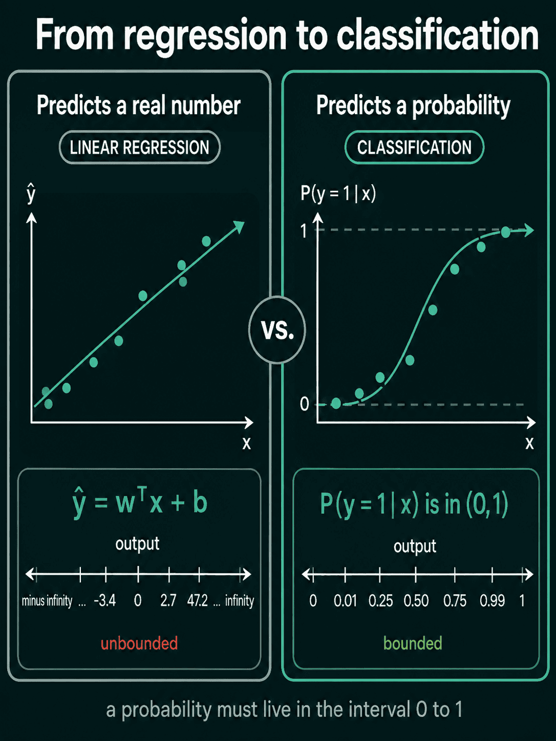
Linear regression predicts a real number from a weighted sum of the inputs. For an input vector $\mathbf{x}$, a weight vector $\mathbf{w}$ with one weight per feature, and one extra number $b$ called the bias, it computes

$$z = \mathbf{w}^\top \mathbf{x} + b$$

$\mathbf{w}^\top \mathbf{x}$ multiplies each feature by its weight and adds the products up. The result $z$ can be any real number, such as -3.4 or 47.2, while a probability has to sit between 0 and 1. Classification needs a function that takes any real number and returns a value between 0 and 1.

Two panels side by side. Left: linear regression, a straight line through points, with an output axis running from minus infinity to infinity, labeled unbounded. Right: classification, an S-shaped curve through points between 0 and 1, with an output axis from 0 to 1, labeled bounded.

The sigmoid function

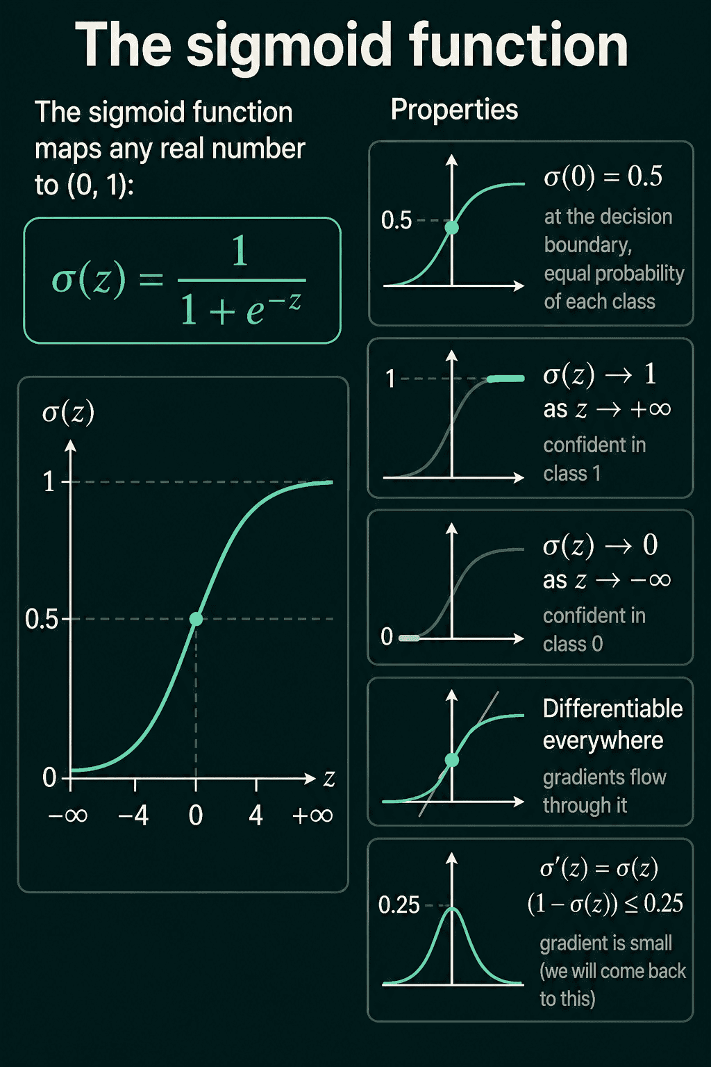
The sigmoid function does that squashing:

$$\sigma(z) = \frac{1}{1 + e^{-z}}$$

When $z$ is large and positive, $e^{-z}$ is close to 0 and $\sigma(z)$ is close to 1. When $z$ is large and negative, $e^{-z}$ is huge and $\sigma(z)$ is close to 0. At $z = 0$, $e^{0} = 1$, so $\sigma(0) = 0.5$, an even split between the two classes.

Sigmoid is smooth, so it has a derivative at every point and gradients can pass through it during training. The derivative has a short form:

$$\sigma'(z) = \sigma(z)\bigl(1 - \sigma(z)\bigr)$$

It peaks at 0.25 when $z = 0$ and shrinks toward 0 as $z$ moves away in either direction. That small derivative decides which loss sigmoid should be trained with, as the gradient section below shows.

The sigmoid curve from 0 to 1 crossing 0.5 at z equals 0, next to four small panels: sigma of 0 is 0.5, sigma goes to 1 as z goes to plus infinity, sigma goes to 0 as z goes to minus infinity, differentiable everywhere, and the derivative sigma times one minus sigma, which peaks at 0.25.

Where sigmoid comes from: log-odds

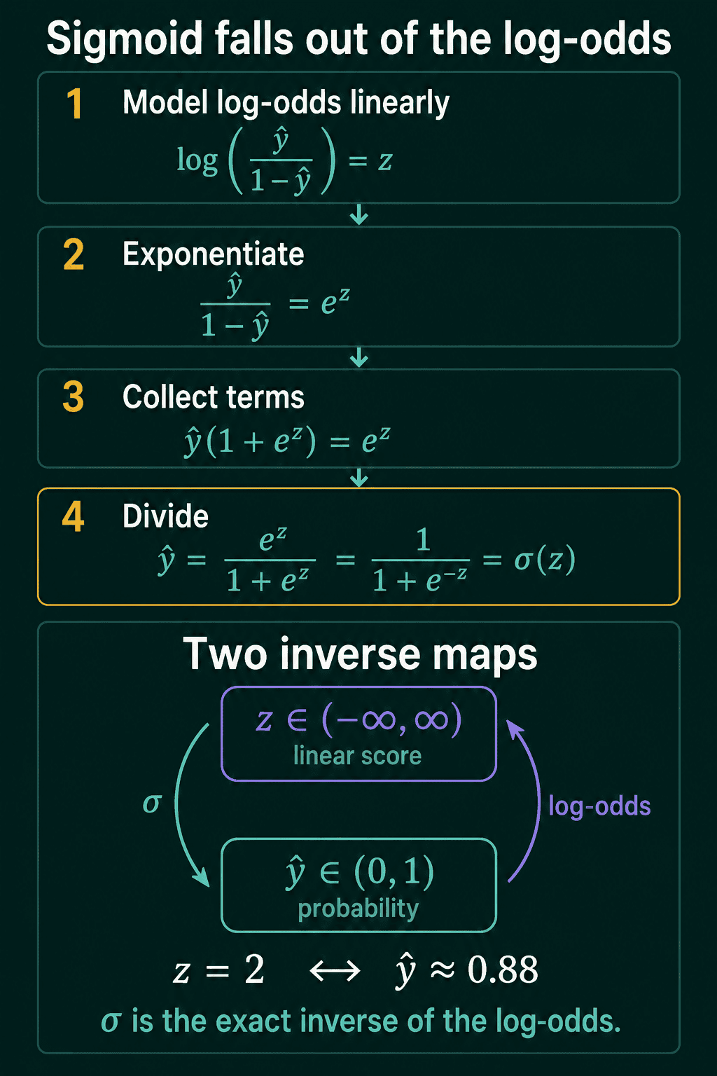
Sigmoid is not an arbitrary pick among S-shaped curves. Write $\hat{y}$ for the model's predicted probability of class 1. The odds of class 1 are $\hat{y} / (1 - \hat{y})$, so a probability of 0.8 gives odds of 4, meaning class 1 is four times as likely as class 0. The log-odds is the natural log of that ratio, and unlike a probability it can take any real value, very negative when class 1 is unlikely and very positive when it is likely.

Logistic regression assumes the log-odds is a linear function of the inputs:

$$\log\frac{\hat{y}}{1 - \hat{y}} = \mathbf{w}^\top \mathbf{x} + b = z$$

Solving for $\hat{y}$ gives the sigmoid. Exponentiating both sides gives $\hat{y}/(1-\hat{y}) = e^{z}$. Multiplying out gives $\hat{y} = e^{z} - e^{z}\hat{y}$, so $\hat{y}(1 + e^{z}) = e^{z}$, and dividing:

$$\hat{y} = \frac{e^{z}}{1 + e^{z}} = \frac{1}{1 + e^{-z}} = \sigma(z)$$

Sigmoid is the inverse of the log-odds, so it turns a linear score back into a probability. A score of $z = 2$ means log-odds of 2, odds of $e^2 \approx 7.4$, and a probability of about 0.88.

Four numbered steps: model the log-odds linearly, exponentiate, collect terms, divide, ending in y hat equals sigma of z. Below, a loop between the linear score z, any real number, and the probability y hat between 0 and 1, with sigma going one way and log-odds the other, and the example z equals 2 maps to y hat of about 0.88.

The logistic regression model

Logistic regression is a linear score followed by a sigmoid:

$$\hat{y} = \sigma(\mathbf{w}^\top \mathbf{x} + b)$$

The raw score $z$ before the sigmoid is called the logit. The model predicts class 1 when $\hat{y} > 0.5$. Training has to find a $\mathbf{w}$ and $b$ that give high $\hat{y}$ on class-1 examples and low $\hat{y}$ on class-0 examples, and for that it needs a loss: one number that measures how wrong the predictions are, which gradient descent then pushes down.

Binary cross-entropy loss

The loss used with logistic regression is binary cross-entropy (BCE). For one example with true label $y$, which is 0 or 1, and predicted probability $\hat{y}$:

$$\mathcal{L} = -\bigl[y \log \hat{y} + (1-y) \log(1-\hat{y})\bigr]$$

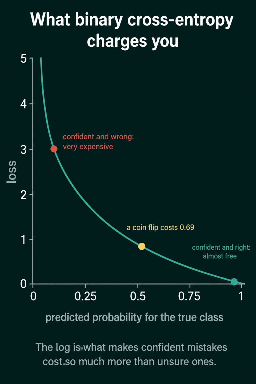
Only one of the two terms is active for each example. When $y = 1$ the loss is $-\log \hat{y}$, and when $y = 0$ it is $-\log(1-\hat{y})$. Both are the negative log of the probability the model gave to the correct class. Over a dataset of $n$ examples, the loss is the average of the $n$ per-example losses.

The log makes confident mistakes expensive. Giving the correct class a probability of 0.95 costs about 0.05. A coin flip, 0.5, costs 0.69. Giving the correct class 0.05, which is confident and wrong, costs about 3.0, and 0.01 costs 4.6. As the probability on the correct class goes to 0, the loss goes to infinity.

The BCE loss plotted against the predicted probability for the true class. It is near 0 at probability 1, marked confident and right: almost free, 0.69 at probability 0.5, marked a coin flip, and climbs steeply toward 5 near probability 0, marked confident and wrong: very expensive.

BCE is not a hand-picked formula. It is the negative log-likelihood of the labels when each label is treated as a biased coin flip that comes up 1 with probability $\hat{y}$, so minimizing BCE is maximum likelihood estimation for this model.

Why sigmoid is paired with cross-entropy and not MSE

Take the derivative of one example's BCE with respect to its logit $z$. By the chain rule it is the derivative of the loss with respect to $\hat{y}$ times the derivative of $\hat{y}$ with respect to $z$:

$$\frac{\partial \mathcal{L}}{\partial \hat{y}} = -\frac{y}{\hat{y}} + \frac{1-y}{1-\hat{y}}$$

$$\frac{\partial \hat{y}}{\partial z} = \hat{y}(1-\hat{y})$$

When the two are multiplied, the $\hat{y}(1-\hat{y})$ factor cancels against the denominators and leaves

$$\frac{\partial \mathcal{L}}{\partial z} = \hat{y} - y$$

The gradient on the logit is the prediction minus the label. A class-1 example predicted at 0.05 gets a gradient of -0.95, a large push toward the right answer. Averaged over $n$ examples, with $\mathbf{X}$ the matrix holding one example per row, the gradients on the parameters are

$$\frac{\partial \mathcal{L}}{\partial \mathbf{w}} = \frac{1}{n}\mathbf{X}^{\top}(\hat{\mathbf{y}} - \mathbf{y})$$

$$\frac{\partial \mathcal{L}}{\partial b} = \frac{1}{n}\sum_{i=1}^{n} (\hat{y}_i - y_i)$$

With mean squared error (MSE) in place of BCE, the cancellation does not happen. The loss for one example is $(\hat{y} - y)^2$, so the gradient on the logit becomes $2(\hat{y} - y),\hat{y}(1-\hat{y})$, and the $\hat{y}(1-\hat{y})$ factor is close to 0 whenever the prediction is close to 0 or 1. The same class-1 example predicted at 0.05 now gets $2 \times (-0.95) \times 0.0475 \approx -0.09$, about ten times smaller, so the model barely moves on the examples it gets most wrong. Sigmoid with BCE also gives logistic regression a convex loss, one with no local minimum other than the lowest point, which sigmoid with MSE does not.

The decision boundary

The model predicts class 1 when $\hat{y} > 0.5$, which happens when $\sigma(z) > 0.5$, which happens when $z > 0$. The border between the two predicted classes is the set of inputs where

$$\mathbf{w}^\top \mathbf{x} + b = 0$$

With two input features that is a straight line, with three it is a flat plane, and in general it is a flat surface called a hyperplane. This border is the decision boundary.

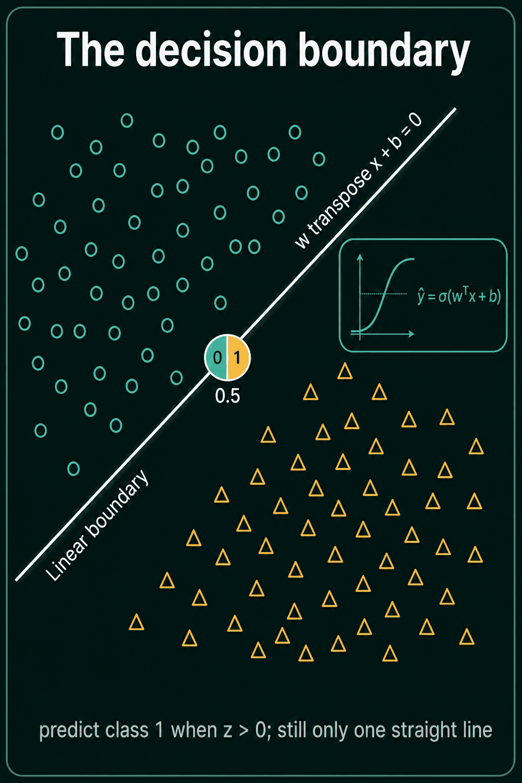
Circles of class 0 in the upper left and triangles of class 1 in the lower right, separated by a straight line labeled w transpose x plus b equals 0, with a 0.5 marker on the line and an inset of the sigmoid. The caption reads: predict class 1 when z is greater than 0, still only one straight line.

Logistic regression can only draw one flat boundary. Classes arranged in a ring, or in opposite corners as in the XOR problem, cannot be split by it with any choice of weights, the same limit as the perceptron.

Why logistic regression is a one-layer neural network

An artificial neuron computes a weighted sum of its inputs plus a bias and passes the result through an activation function. Logistic regression is one neuron with sigmoid as the activation, with no hidden layers. In PyTorch it is one nn.Linear layer with one output. A neural network for a yes/no task usually keeps the same last step, one output logit trained with BCE, and puts hidden layers in front of it. The hidden layers turn the inputs into new features where the two classes can be split by the one flat boundary the output neuron draws.

Logistic regression in PyTorch

This script trains logistic regression on two clusters of 200 points each:

1import torch
2from torch import nn
3 
4torch.manual_seed(0)
5 
6# class 0 is centered at (-2, -2), class 1 at (2, 2)
7n = 200
8x0 = torch.randn(n, 2) + torch.tensor([-2.0, -2.0])
9x1 = torch.randn(n, 2) + torch.tensor([2.0, 2.0])
10X = torch.cat([x0, x1])                                   # shape (400, 2)
11y = torch.cat([torch.zeros(n, 1), torch.ones(n, 1)])      # shape (400, 1), float labels
12 
13model = nn.Linear(in_features=2, out_features=1)          # w has 2 entries, b has 1
14loss_fn = nn.BCEWithLogitsLoss()                          # sigmoid and BCE in one step
15optimizer = torch.optim.SGD(model.parameters(), lr=0.1)
16 
17for epoch in range(200):
18    optimizer.zero_grad()
19    logits = model(X)                                     # shape (400, 1), the raw scores z
20    loss = loss_fn(logits, y)
21    loss.backward()
22    optimizer.step()
23 
24probs = torch.sigmoid(model(X))                           # probabilities in (0, 1)
25preds = (probs > 0.5).float()
26accuracy = (preds == y).float().mean().item()
27print(f"loss {loss.item():.3f}, accuracy {accuracy:.3f}")
28print("w:", model.weight.data, "b:", model.bias.data)

The model returns logits and has no sigmoid inside, because nn.BCEWithLogitsLoss applies the sigmoid itself. Sigmoid appears only after training, to turn logits into probabilities. The loss ends at a few hundredths, the accuracy close to 1.0, and the two weights come out positive and similar in size with a bias near 0, since the boundary runs diagonally between the two clusters. If the loss stays flat on real data, standardizing the features and lowering the learning rate by a factor of 10 are the first two things to try.

BCEWithLogitsLoss vs BCELoss

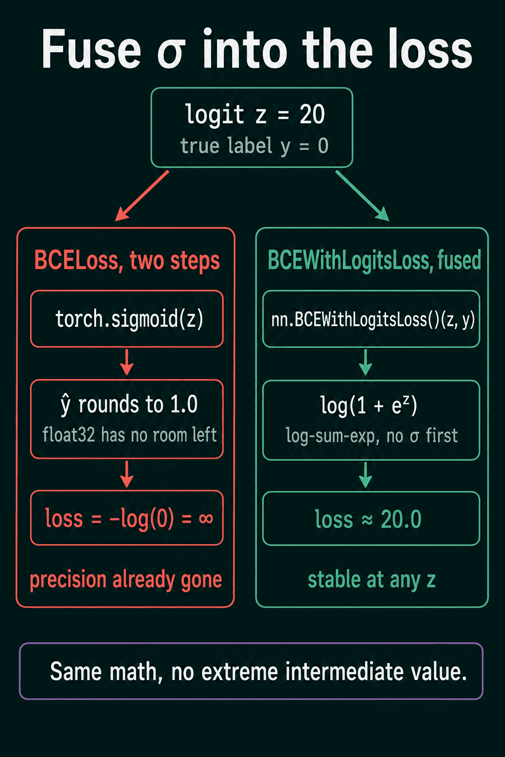
PyTorch has two BCE losses. nn.BCELoss takes probabilities, so the model has to apply sigmoid first. nn.BCEWithLogitsLoss takes logits and applies the sigmoid inside the loss, and it is the one to use by default.

The two-step version loses precision at large logits. Take a logit of $z = 20$ on an example whose label is $y = 0$. $\sigma(20)$ is about $1 - 2 \times 10^{-9}$, and a 32-bit float cannot store a number that close to 1, so it rounds to exactly 1.0. The loss then needs $-\log(1 - 1.0) = -\log(0)$, which is infinite. BCELoss clamps the log at -100 to avoid the infinity, so it reports a loss of 100 where the correct value is about 20. BCEWithLogitsLoss rewrites this loss as $\log(1 + e^{z})$ and computes it with the log-sum-exp trick, a rearrangement that never forms $\sigma(z)$, so it returns 20.0.

A logit z of 20 with true label 0 goes down two paths. BCELoss, two steps: torch.sigmoid rounds y hat to 1.0 in float32, then the loss is minus log of 0, infinity, labeled precision already gone. BCEWithLogitsLoss, fused: computes log of 1 plus e to the z with log-sum-exp and no sigmoid first, loss about 20.0, stable at any z.

When to use logistic regression, and common mistakes

Logistic regression is a good first model for a yes/no problem on tabular data. It trains in seconds, and each weight says how much its feature raises or lowers the log-odds, which makes the model easy to inspect. It is worth training before a neural network, because a larger model that does not beat it has not found anything the flat boundary missed. It stops being enough when the classes cannot be separated by a flat boundary and no hand-made feature fixes that.

Common mistakes:

Applying sigmoid twice. A torch.sigmoid inside the model's forward followed by BCEWithLogitsLoss squashes the outputs twice. Training runs without an error, but the loss sees inputs between 0 and 1, so its implied probabilities stay between 0.5 and 0.73 and the model can never become confident.
Labels with the wrong shape or type. BCEWithLogitsLoss expects float labels with the same shape as the logits, such as (batch_size, 1). Integer labels raise an error, and labels of shape (batch_size,) against logits of shape (batch_size, 1) raise a size mismatch error.
Unscaled features. A feature measured in thousands next to one measured in fractions gives one weight huge gradients and the other tiny ones. Standardizing each feature to mean 0 and standard deviation 1 usually fixes slow or unstable training.
Treating 0.5 as the only threshold. 0.5 is the default cut. When a missed positive costs more than a false alarm, a lower threshold such as 0.3 catches more positives, and it is chosen on validation data after training.
Ignoring class imbalance. With 1 positive per 100 examples, predicting 0 everywhere scores 99% accuracy. nn.BCEWithLogitsLoss(pos_weight=torch.tensor([99.0])) counts each positive example 99 times, and precision and recall say more than accuracy about how the model is doing.

Softmax extends logistic regression to more than two classes, with one logit per class, softmax in place of sigmoid, and cross-entropy in place of BCE. Multi-label classification, where one input can have several labels at once, uses one sigmoid and one BCE term per label. The perceptron computes the same weighted sum but outputs a hard 0 or 1 in place of a probability, so it has no gradient to train with. A multilayer perceptron puts hidden layers in front of a logistic output and can draw curved boundaries.

QuiddityML teaches sigmoid, logistic regression, and binary cross-entropy as three concepts in the ML Foundation track, with exercises that include writing sigmoid without torch.sigmoid, spotting the buggy line in a logistic regression module, and writing BCE with the clamp that keeps log(0) out of the loss.