26 September 2026 · 8 min read
Maximum likelihood estimation explained: where MSE and cross-entropy come from
Maximum likelihood estimation picks the model parameters that make the observed data most probable. This post explains it with a coin-flip example, then shows how the same idea produces mean squared error for regression and cross-entropy for classification.
Maximum likelihood estimation (MLE) picks the model parameters that make the data you actually observed as probable as possible. It also explains why regression models usually train on mean squared error and classifiers on cross-entropy: both losses come out of MLE once you say what kind of randomness you expect in the labels. Knowing that link tells you what a loss assumes about your data, and what to switch to when the assumption is wrong.
A coin example
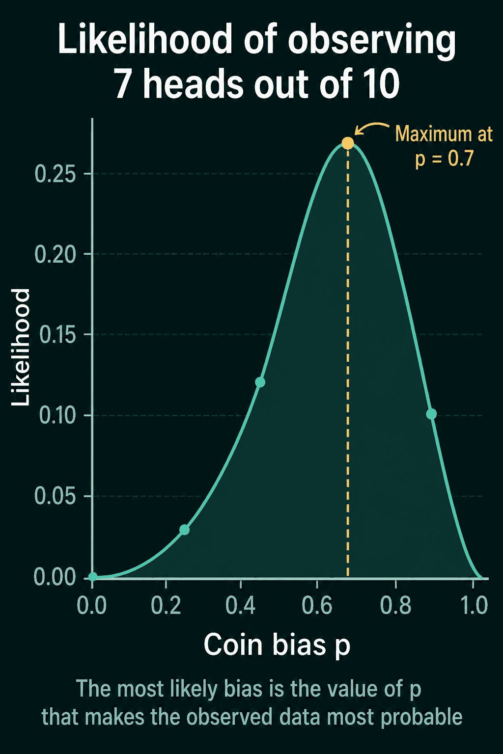
Flip a coin 10 times and get 7 heads. Call the coin's probability of heads $p$, its bias. MLE asks which value of $p$ makes this result most probable.
For any candidate $p$, the probability of getting exactly 7 heads in 10 flips is
$$P(7 \text{ heads}) = \binom{10}{7}, p^7 (1-p)^3$$
where $\binom{10}{7} = 120$ counts the orders the 7 heads could come in. Plug in a few values: $p = 0.5$ gives 0.117, $p = 0.7$ gives 0.267, and $p = 0.9$ gives 0.057. Read as a function of $p$, with the 7 heads held fixed, this curve is called the likelihood, and the $p$ at its peak is the maximum likelihood estimate. Here the peak sits at $p = 0.7$, the share of heads in the data.
Likelihood vs probability
In a model, the parameters are the weights and biases that training adjusts, written together as $\theta$ (theta). An input is $x$ and its label is $y$.
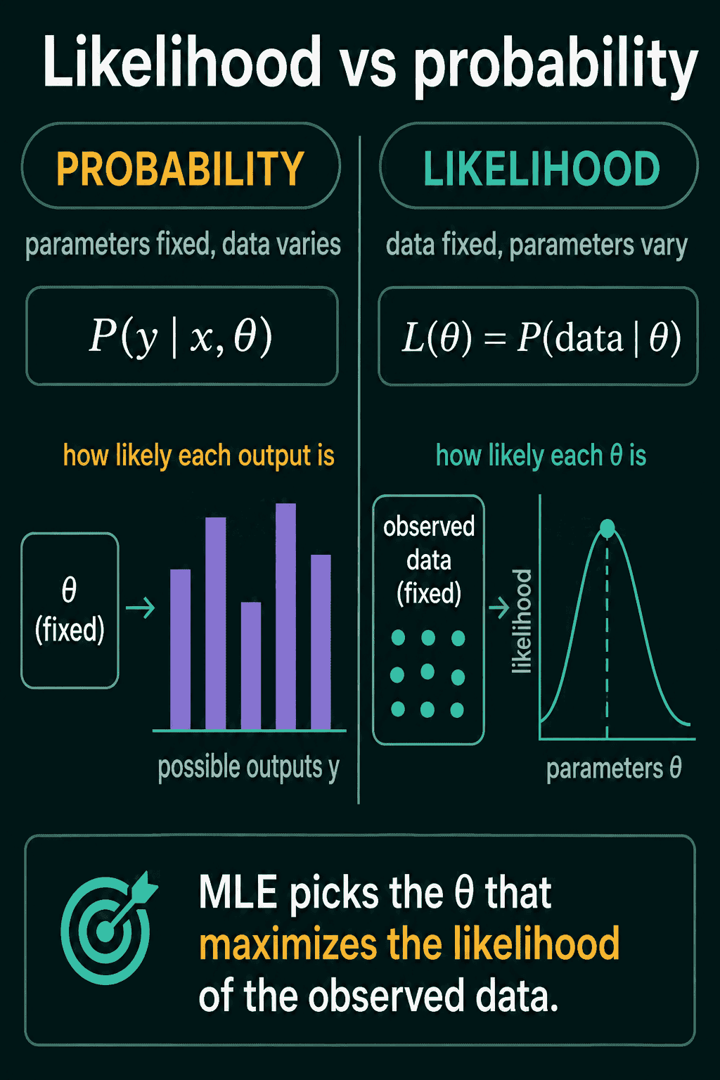
Probability and likelihood use the same formula and read it in opposite directions. Probability holds $\theta$ fixed and asks how likely each possible output is:
$$P(y \mid x, \theta)$$
Likelihood holds the observed data fixed and asks how well each value of $\theta$ explains it:
$$L(\theta) = P(\text{data} \mid \theta)$$
The coin curve is a likelihood: the 7 heads stayed fixed and $p$ moved along the horizontal axis. MLE searches for the $\theta$ that makes $L(\theta)$ as large as possible. Note the letter: $L$ is the likelihood, which you want large, and a loss, written $\mathcal{L}$, is something you want small.
From likelihood to negative log-likelihood
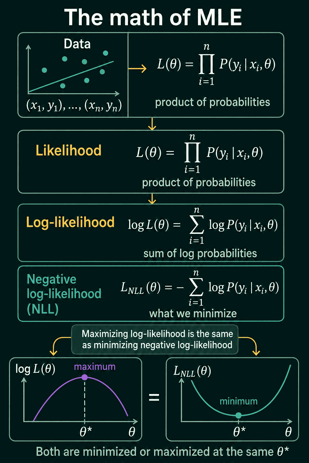
A dataset has $n$ examples $(x_1, y_1), \dots, (x_n, y_n)$. MLE usually assumes they are i.i.d., independent and identically distributed: one example tells you nothing about another, and they come from the same data-collecting process. Under that assumption, the probability of the whole dataset is the product of the per-example probabilities:
$$L(\theta) = \prod_{i=1}^{n} P(y_i \mid x_i, \theta)$$
Multiplying thousands of numbers below 1 breaks floating point arithmetic. A model that gives 1,000 examples probability 0.9 each has likelihood $0.9^{1000} \approx 1.7 \times 10^{-46}$, and in float32 that product comes out as exactly 0. Taking the log turns the product into a sum, and the sum of those 1,000 logs is a manageable $-105.4$:
$$\log L(\theta) = \sum_{i=1}^{n} \log P(y_i \mid x_i, \theta)$$
The log is an increasing function, so the $\theta$ that maximizes $\log L(\theta)$ also maximizes $L(\theta)$. Gradient descent is built to minimize, so the last step flips the sign. The result is the negative log-likelihood (NLL):
$$\mathcal{L}{\text{NLL}}(\theta) = -\sum{i=1}^{n} \log P(y_i \mid x_i, \theta)$$
The parameters MLE is looking for, written $\theta^*$, sit at the top of the log-likelihood and at the bottom of the NLL. Training a model by MLE means minimizing this sum.
So far $P(y_i \mid x_i, \theta)$ has no formula. Choosing one is choosing a distribution for the labels, and that choice decides which loss comes out.
Where MSE comes from
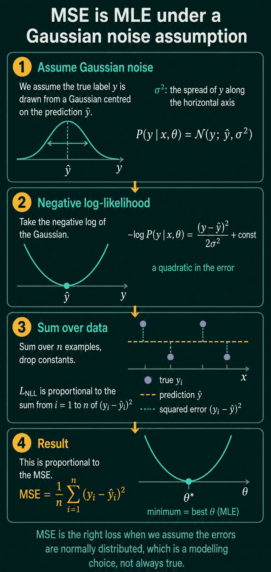
In regression the label $y$ is a number, and the model predicts $\hat y$ (read "y-hat"). The usual assumption is that $y$ equals $\hat y$ plus random noise from measurement error, missing features, and plain randomness, and that the noise follows a Gaussian (normal) distribution: a bell curve centred on $\hat y$ where small errors are common and large ones are rare. Its spread is set by the variance $\sigma^2$:
$$P(y \mid x, \theta) = \mathcal{N}(y;, \hat y, \sigma^2)$$
$$= \frac{1}{\sqrt{2\pi\sigma^2}} \exp!\left(-\frac{(y - \hat y)^2}{2\sigma^2}\right)$$
Taking the negative log removes the exponential:
$$-\log P(y \mid x, \theta) = \frac{(y - \hat y)^2}{2\sigma^2} + \tfrac{1}{2}\log(2\pi\sigma^2)$$
If $\sigma$ is a fixed number, the second term is a constant and $\frac{1}{2\sigma^2}$ is a constant multiplier, and neither changes which $\theta$ gives the minimum. Drop both, sum over the $n$ examples, divide by $n$, and what remains is mean squared error:
$$\text{MSE} = \frac{1}{n}\sum_{i=1}^{n}(y_i - \hat y_i)^2$$
Minimizing MSE is MLE under the assumption that the errors are Gaussian with a fixed spread. It also explains why a model trained on MSE predicts the average of the possible $y$ values for a given input: the number that minimizes the average squared distance to a set of values is their mean.
Where cross-entropy comes from
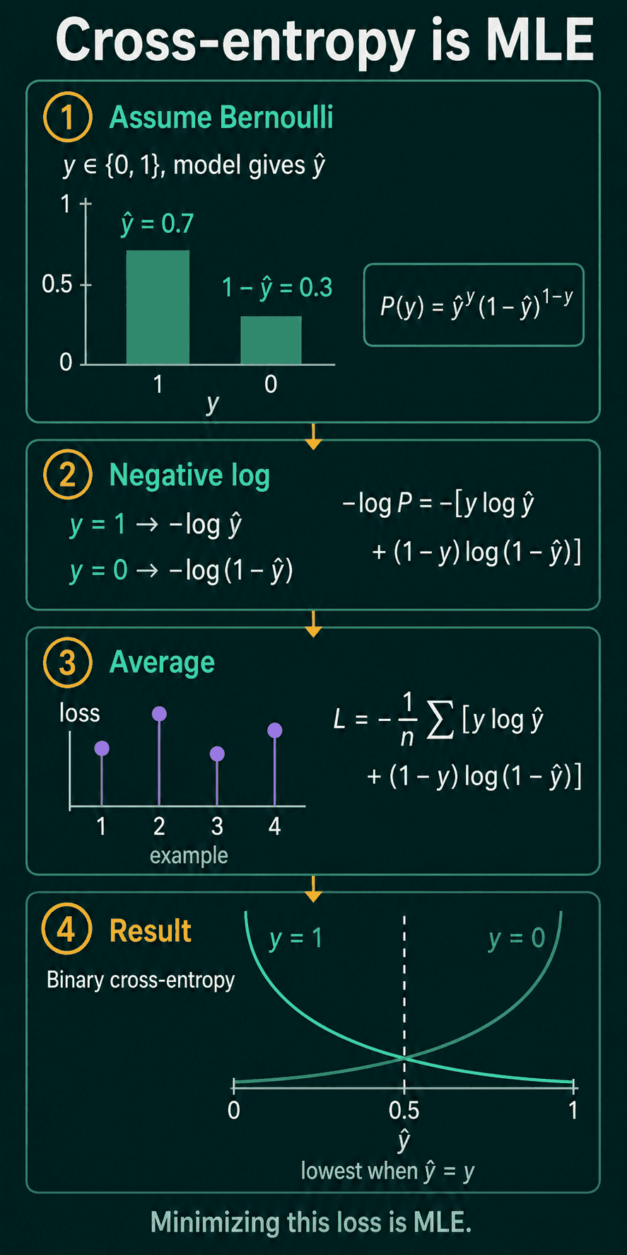
In binary classification the label $y$ is 0 or 1, and the model outputs $\hat y$, the probability that $y = 1$. An outcome with two possible values and one probability follows a Bernoulli distribution:
$$P(y \mid x, \theta) = \hat y^{,y} (1 - \hat y)^{1-y}$$
That formula is a compact way of writing two cases. With $\hat y = 0.7$, a label of 1 gets probability 0.7 and a label of 0 gets 0.3. The negative log is
$$-\log P = -\bigl[y \log \hat y + (1-y)\log(1 - \hat y)\bigr]$$
For $\hat y = 0.7$ that costs $-\log 0.7 = 0.357$ when the label is 1 and $-\log 0.3 = 1.204$ when it is 0. Averaging over the $n$ examples gives binary cross-entropy:
$$\text{BCE} = -\frac{1}{n}\sum_{i=1}^{n}\bigl[y_i \log \hat y_i + (1-y_i)\log(1-\hat y_i)\bigr]$$
The loss is smallest when $\hat y$ matches the label and climbs steeply as $\hat y$ moves toward the wrong end.
With $K$ classes, the model outputs $K$ probabilities that sum to 1, a categorical distribution, which is the Bernoulli extended past two outcomes. The probability of the observed label is the probability given to the correct class, so the NLL is $-\log$ of that number, averaged over examples. That is multi-class cross-entropy, what nn.CrossEntropyLoss computes. The cross-entropy loss post looks at the same loss through entropy and KL divergence.
Which assumption each loss makes
The same recipe works for other distributions. Laplace noise has a sharper peak and heavier tails than a Gaussian, with density proportional to $\exp(-|y - \hat y|/b)$ for a fixed width $b$. Its negative log is $|y - \hat y|/b$ plus a constant, which is mean absolute error (MAE) up to scaling. The number that minimizes the average absolute distance to a set of values is their median, so a model trained on MAE predicts the median.
| loss | assumed distribution of y | model predicts |
|---|---|---|
| MSE | Gaussian around the prediction | the mean |
| MAE | Laplace around the prediction | the median |
| binary cross-entropy | Bernoulli | probability of class 1 |
| cross-entropy | categorical | one probability per class |
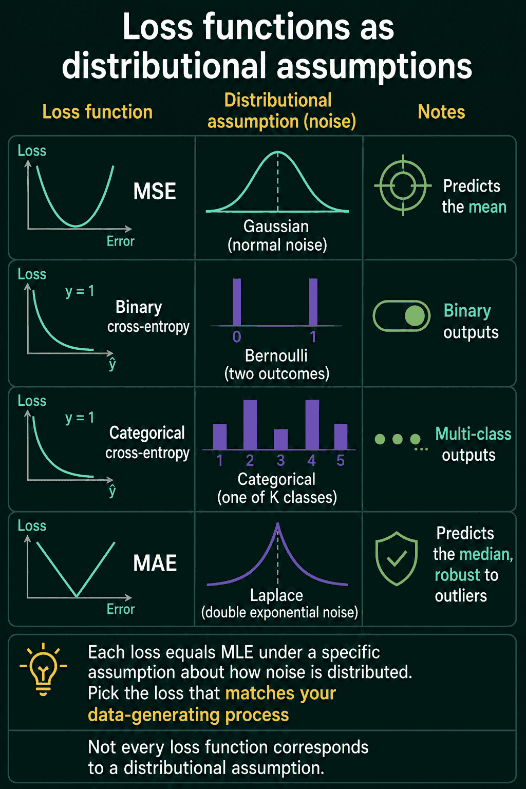
Picking a loss is a statement about how your labels were generated. MSE says large errors are rare, so an error 10 times larger costs 100 times more. With heavy-tailed noise, such as a few mislabelled prices, that statement is wrong and MAE or Huber loss fits better. Huber is squared for small errors and absolute for large ones, a Gaussian core with Laplace tails. Some losses, such as hinge loss and focal loss, have no clean MLE reading.
MLE in PyTorch
The coin example can be solved with gradient descent on the NLL. The parameter is a logit, a raw number passed through a sigmoid, so $p$ stays between 0 and 1 while the logit moves freely:
1import torch
2
3flips = torch.tensor([1., 1., 0., 1., 1., 0., 1., 1., 0., 1.])  # 7 heads, 3 tails
4logit = torch.zeros(1, requires_grad=True)  # sigmoid(0) = 0.5, a fair coin
5opt = torch.optim.SGD([logit], lr=0.1)
6
7for step in range(200):
8    p = torch.sigmoid(logit)
9    nll = -(flips * torch.log(p) + (1 - flips) * torch.log(1 - p)).sum()
10    opt.zero_grad()
11    nll.backward()
12    opt.step()
13
14print(torch.sigmoid(logit).item())  # 0.7
After 200 steps $p$ reaches 0.7, the peak of the likelihood curve, and the NLL there is 6.11.
The second snippet checks both derivations. With a variance of 1, Gaussian NLL equals half the MSE plus $\tfrac{1}{2}\log 2\pi \approx 0.919$, and the hand-written NLL matches F.cross_entropy:
1import torch
2import torch.nn as nn
3import torch.nn.functional as F
4
5# Regression: Gaussian NLL with variance 1 is half the MSE plus a constant
6pred = torch.tensor([2.5, 0.0, 2.1])
7target = torch.tensor([3.0, -0.5, 2.0])
8gauss_nll = nn.GaussianNLLLoss(full=True)(pred, target, torch.ones(3))
9print(F.mse_loss(pred, target))                 # 0.17
10print(gauss_nll)                                # 1.0039
11print(0.5 * F.mse_loss(pred, target) + 0.9189)  # 1.0039
12
13# Classification: NLL of the true class is cross-entropy
14logits = torch.tensor([[2.0, 0.5, -1.0], [0.1, 1.5, 0.3]])
15targets = torch.tensor([0, 2])
16log_probs = F.log_softmax(logits, dim=1)
17nll = -log_probs[torch.arange(len(targets)), targets].mean()
18print(nll)                                      # 0.9391
19print(F.cross_entropy(logits, targets))         # 0.9391
log_probs[torch.arange(len(targets)), targets] picks one entry per row, the log-probability of that row's true class. Writing log_probs[:, targets] instead returns an $n \times n$ block, a common reason a hand-written NLL disagrees with the built-in one.
When the MLE view helps, and common mistakes
The MLE view helps when choosing a loss for a new kind of target. Ask what distribution the label plausibly follows around the model's prediction, then take its negative log. Counts such as clicks per hour suggest a Poisson distribution, and PyTorch has nn.PoissonNLLLoss for it. If the noise level changes from input to input, the model can predict $\sigma^2$ alongside $\hat y$ and train on nn.GaussianNLLLoss instead of plain MSE.
Mistakes that show up often:
- Passing probabilities to
nn.NLLLoss. It expects log-probabilities, usually fromF.log_softmax, and returns wrong values on plain probabilities without raising an error. - Switching between sum and mean. The NLL above is a sum, while PyTorch losses average by default. Both have the same minimum, but the sum scales the gradient by $n$, so a learning rate tuned for one does not carry over to the other.
- Trusting MLE on very little data. Three flips that land heads give an estimate of $p = 1$, a coin with zero chance of tails. With a small sample, fitting it exactly is overfitting. A penalty on the weights, as in regularization, is a common fix.
Related concepts
The loss function post covers which loss to pick for each task and the PyTorch class for each. Gradient descent is the algorithm that minimizes the NLL once MLE has written it down. Linear regression from scratch trains a model on MSE, which by the derivation above is MLE with Gaussian noise. MAP estimation (maximum a posteriori) is a close relative of MLE: it adds a prior belief about the parameters to the likelihood, and a Gaussian prior on the weights turns into an L2 penalty added to the loss.
QuiddityML teaches maximum likelihood estimation in the first unit of its ML Foundation track, right before gradient descent, and the exercises on it include writing negative log-likelihood from its equation with torch.arange indexing, finding a .mean() that should be a .sum(), and predicting the error when a target class index is out of range.