26 September 2026 · 8 min read

The PyTorch training loop explained, with Dataset and DataLoader

The training loop is the five lines of PyTorch code that make a model learn from data. This post explains what each line does, why their order can't be swapped, and how a Dataset and DataLoader feed the loop one batch at a time.

A training loop is the code that makes a model learn: it shows the model a small group of examples, measures how wrong its predictions are, adjusts the model so they become less wrong, and repeats. In PyTorch it is five lines inside a loop, and most PyTorch models, from linear regression to large language models, train with those same five lines. Two PyTorch classes, Dataset and DataLoader, cut the training data into groups and hand them to the loop one at a time.

The four pieces a model needs to learn

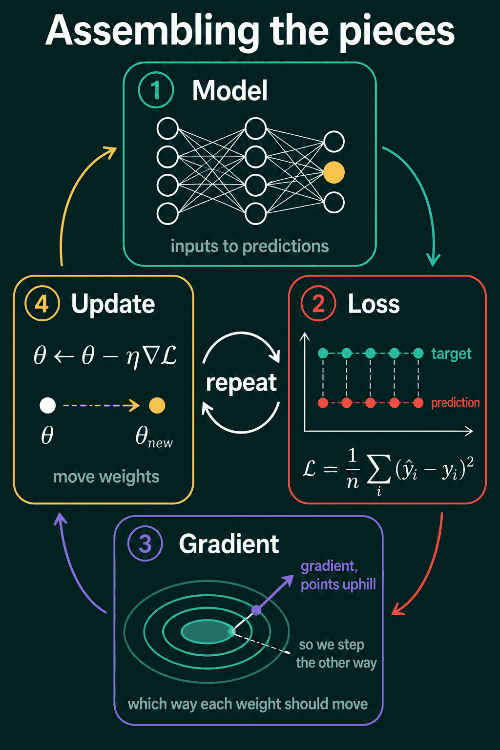
A model is a function with adjustable numbers inside it, called weights or parameters. Training changes those numbers so the predictions get closer to the right answers, which takes four pieces:

1. A model, which turns inputs into predictions.
2. A loss function, which turns the predictions and the true answers into one number that says how wrong the predictions are. Lower is better.
3. A gradient, which says, for each weight, how much the loss would go up if that weight went up slightly.
4. An update rule, which moves each weight in the direction that lowers the loss.

A common loss for predicting numbers is mean squared error (MSE). For $n$ examples with predictions $\hat y_i$ and true values $y_i$, it averages the squared differences:

$$\mathcal{L} = \frac{1}{n}\sum_i (\hat y_i - y_i)^2$$

The gradient points toward higher loss, so the update rule steps the other way. Write the weights as $\theta$, the gradient of the loss as $\nabla \mathcal{L}$, and a small positive step size called the learning rate as $\eta$. The plain gradient descent rule is:

$$\theta \leftarrow \theta - \eta \nabla \mathcal{L}$$

The arrow means the old weights are replaced by the new ones, so each weight moves a small step against its own gradient (gradient descent has the details). The training loop runs these four pieces in a cycle.

The five lines of a PyTorch training loop

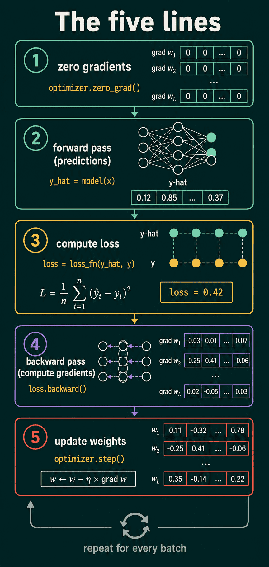
1for x, y in dataloader:
2    optimizer.zero_grad()      # 1. clear old gradients
3    y_hat = model(x)           # 2. forward pass: compute predictions
4    loss = loss_fn(y_hat, y)   # 3. compute loss
5    loss.backward()            # 4. backward pass: compute gradients
6    optimizer.step()           # 5. update weights

Here x is a batch of inputs, y holds their true answers, and optimizer is the object that applies the update rule. One run of the loop body is one training step. The model, the loss and the optimizer change from project to project, and these five lines usually stay the same. Line 1 is easier to follow after the other four, so it comes last below.

Forward pass: y_hat = model(x)

The model computes predictions for the batch with its current weights. Nothing is learned on this line.

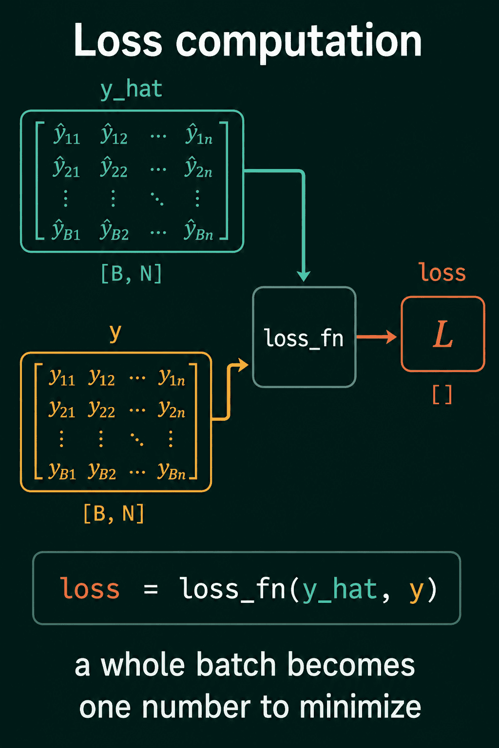
Loss: loss = loss_fn(y_hat, y)

The loss function compares the predictions with the true answers and collapses the whole batch into one number. If a batch has $B$ examples with $N$ outputs each, y_hat and y both have shape [B, N], and loss has shape [], a tensor with no dimensions that holds a single value. This is the number the other lines exist to push down.

Backward pass: loss.backward()

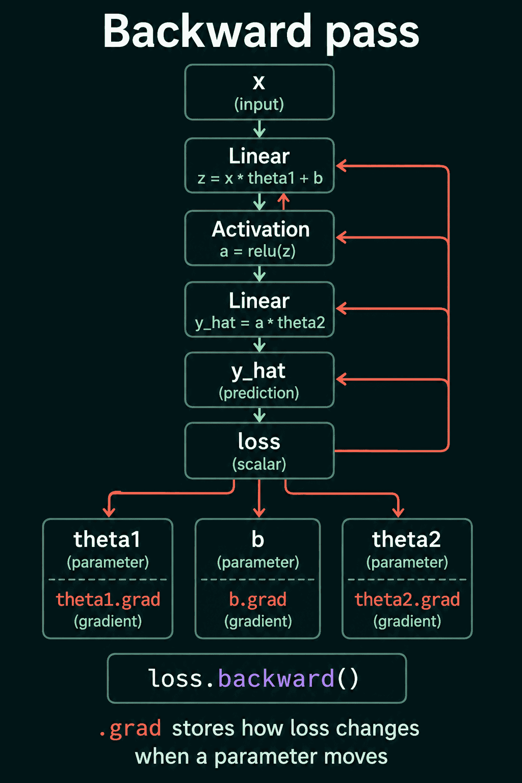
Starting from the loss, PyTorch walks back through each operation that produced it, applying the chain rule from calculus at each one, and stores each weight's gradient in that weight's .grad attribute. This procedure is called backpropagation. For a network made of a linear layer ($z = x\theta_1 + b$), a ReLU (which turns negative values into 0) and a second linear layer ($\hat y = a\theta_2$), one call fills in theta1.grad, b.grad and theta2.grad.

Weight update: optimizer.step()

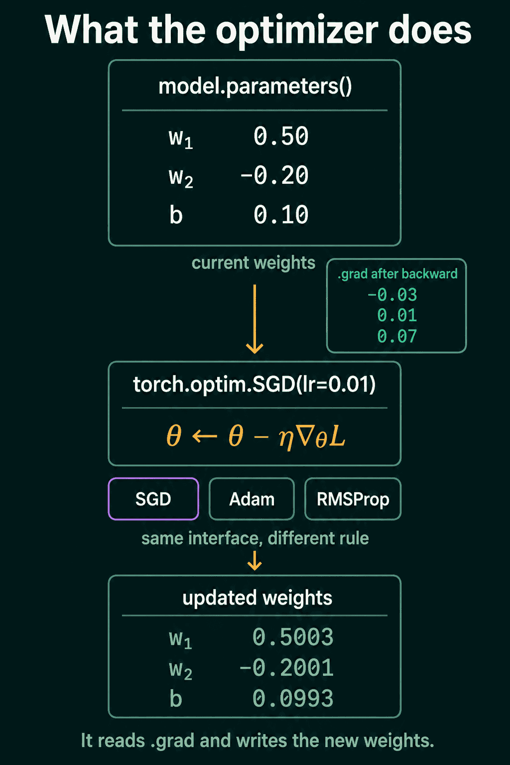
The optimizer is created once, before the loop, and told which tensors it may change:

1optimizer = torch.optim.SGD(model.parameters(), lr=0.01)

model.parameters() hands it the model's weights, and lr=0.01 is the learning rate $\eta$. SGD (stochastic gradient descent) applies the plain update rule above: each step() subtracts lr times .grad from each weight. With weights $w_1 = 0.50$, $w_2 = -0.20$ and bias $b = 0.10$, and gradients of $-0.03$, $0.01$ and $0.07$, the new values are $0.50 - 0.01 \times (-0.03) = 0.5003$, then $-0.2001$ and $0.0993$. Adam and RMSProp use the same step() call with a different update rule, so switching optimizers is a one-line change.

Clearing gradients: optimizer.zero_grad()

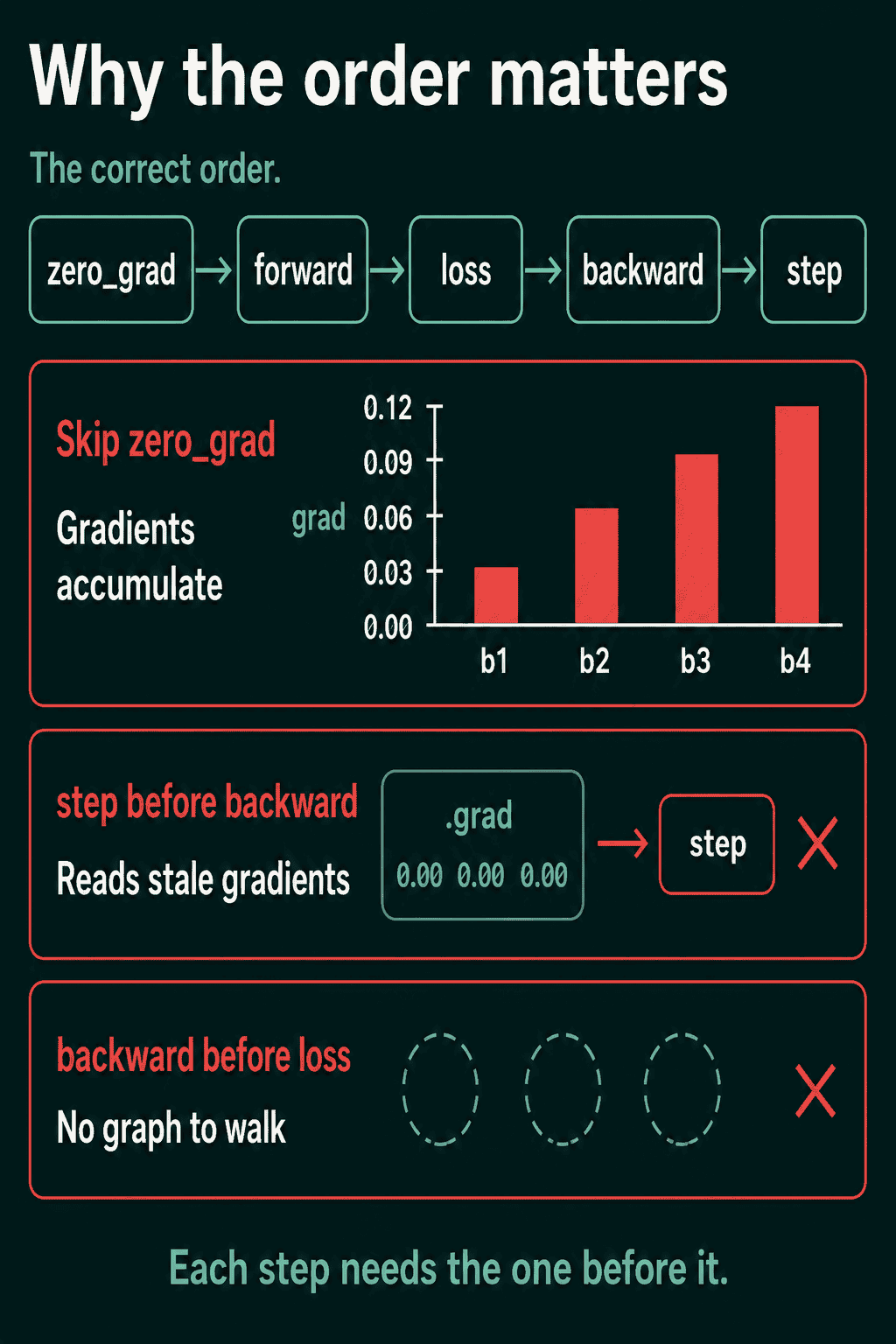
PyTorch adds each new gradient to whatever is already in .grad instead of overwriting it, so without a reset the fourth batch's update would use the sum of the gradients from batches one through four. optimizer.zero_grad() clears .grad at the start of each step.

What goes wrong when the order changes

Each line depends on something an earlier line left behind, and a swap often breaks training without any error message.

• Skipping zero_grad(). Gradients pile up across batches, and each update mixes in directions from old batches.
• step() before backward(). step() uses whatever .grad holds at that moment, which is empty right after zero_grad() or left over from the previous batch. The weights move the wrong way or stay put, and PyTorch raises no error.
• backward() before the loss. backward() walks the chain of operations that produced the loss tensor, so with no loss there is nothing for it to walk.

Batches and epochs

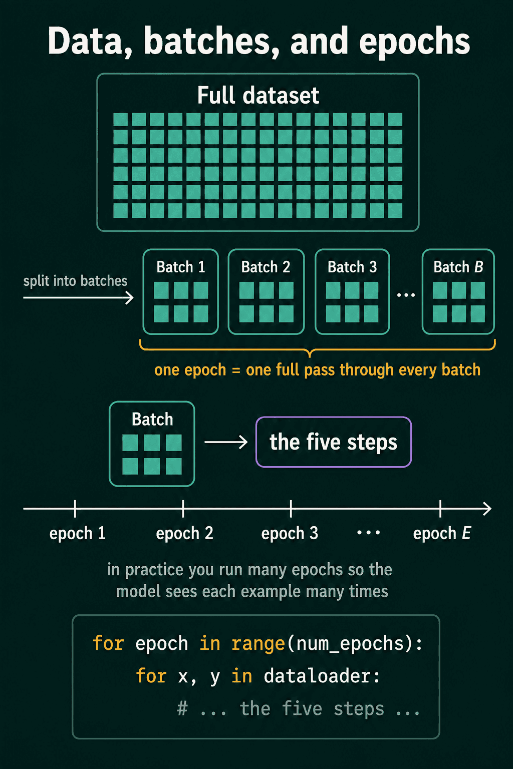
The data is split into batches, small groups of examples, and each training step processes one batch. One epoch is one full pass over the training set. Training usually runs for many epochs, which adds an outer loop:

1for epoch in range(num_epochs):
2    for x, y in dataloader:
3        ...  # the five lines

With 1,000 examples and a batch size of 32, one epoch is 32 steps: 31 full batches and a last batch of 8. Ten epochs means 320 weight updates.

What Dataset and DataLoader do

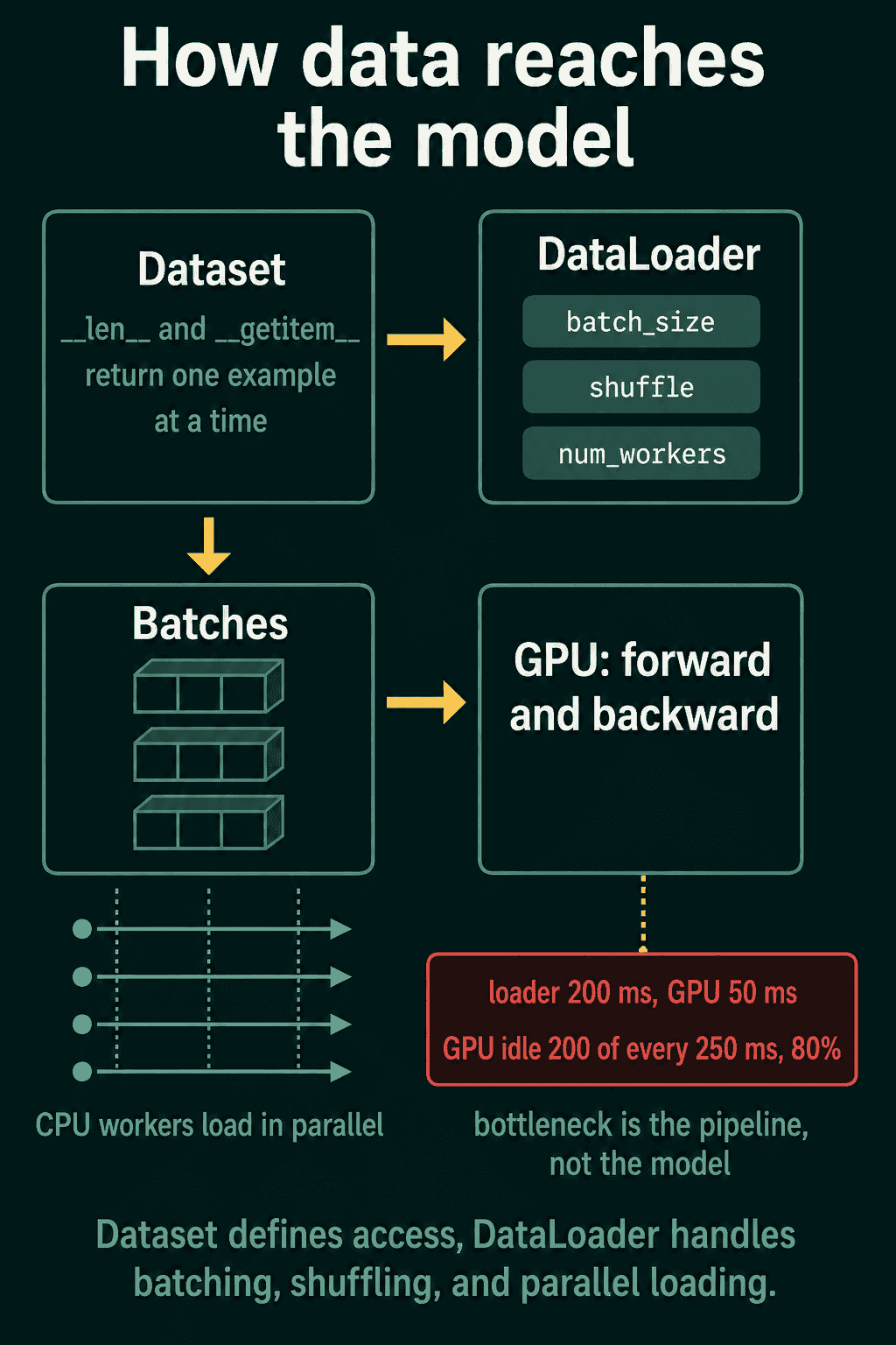
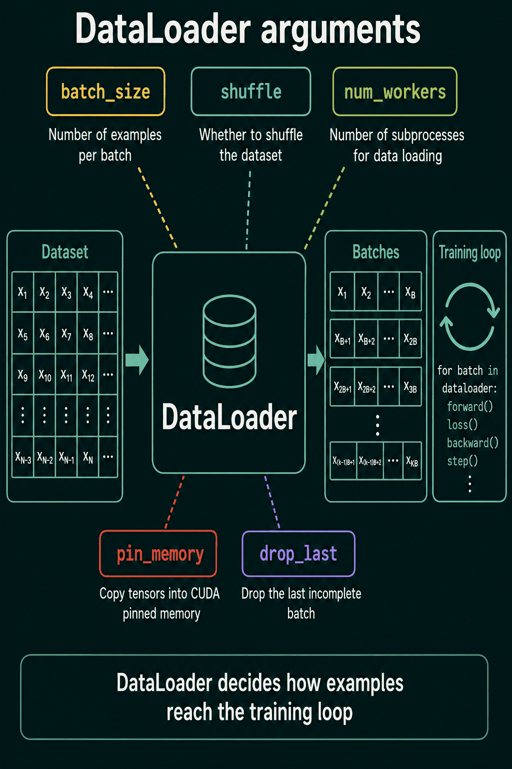
Training data is often too large to fit in memory at once, and GPU memory is smaller still, so PyTorch splits the job of feeding batches between two classes. A Dataset knows how to fetch one example. A DataLoader wraps a Dataset, groups examples into batches, reshuffles their order each epoch, and can prepare batches in parallel.

To write a Dataset, subclass torch.utils.data.Dataset and implement two methods:

1import torch
2from torch.utils.data import Dataset, DataLoader
3 
4class MyDataset(Dataset):
5    def __init__(self, data, labels):
6        self.data = data
7        self.labels = labels
8 
9    def __len__(self):
10        return len(self.data)
11 
12    def __getitem__(self, idx):
13        return self.data[idx], self.labels[idx]
14 
15X = torch.randn(1000, 2)
16y = torch.randn(1000, 1)
17dataset = MyDataset(X, y)
18print(len(dataset))           # 1000
19print(dataset[0][0].shape)    # torch.Size([2])
20 
21loader = DataLoader(dataset, batch_size=32, shuffle=True)
22print(len(loader))            # 32
23x_batch, y_batch = next(iter(loader))
24print(x_batch.shape, y_batch.shape)  # torch.Size([32, 2]) torch.Size([32, 1])

__len__ returns the number of examples, which tells the DataLoader when an epoch ends. __getitem__ returns one example for a given index. With shuffle=True, the DataLoader asks for indices in a new random order each epoch and stacks 32 inputs of shape [2] into one tensor of shape [32, 2]. Reading a file from disk and preprocessing one example usually go inside __getitem__.

Loading runs once per batch inside the loop. If the GPU needs 50 ms for a batch and the loader needs 200 ms to prepare the next one, each step takes 250 ms and the GPU sits idle for 200 of them, 80% of the time. Worker processes help by preparing the next batches on the CPU while the GPU works.

DataLoader arguments

• batch_size: examples per batch, and so per weight update. Larger batches keep the hardware busier and use more memory.
• shuffle: True for training, so the model can't learn from the order of the rows, False for evaluation.
• num_workers: how many CPU processes load data in parallel, with 0 loading in the main process. A good value depends on the machine, so timing one epoch with 2, 4 and 8 workers is a quick way to pick one.
• pin_memory: True puts batches in pinned (page-locked) memory, which can speed up copying them to a CUDA GPU.
• drop_last: True drops a final batch smaller than batch_size, which helps layers that compute statistics over the batch, since a leftover batch of one example gives a poor variance estimate.

A complete training loop in PyTorch

This script trains a linear model on 1,000 synthetic examples generated from $y = 2x_1 - 3x_2 + 1$ plus a little noise:

1import torch
2import torch.nn as nn
3from torch.utils.data import Dataset, DataLoader
4 
5torch.manual_seed(0)
6 
7# Synthetic data: y = 2*x1 - 3*x2 + 1, plus a little noise
8X = torch.randn(1000, 2)
9y = X @ torch.tensor([[2.0], [-3.0]]) + 1.0 + 0.1 * torch.randn(1000, 1)
10 
11 
12class MyDataset(Dataset):
13    def __init__(self, data, labels):
14        self.data = data
15        self.labels = labels
16 
17    def __len__(self):
18        return len(self.data)
19 
20    def __getitem__(self, idx):
21        return self.data[idx], self.labels[idx]
22 
23 
24train_loader = DataLoader(MyDataset(X, y), batch_size=32, shuffle=True)
25 
26model = nn.Linear(in_features=2, out_features=1)
27loss_fn = nn.MSELoss()
28optimizer = torch.optim.SGD(model.parameters(), lr=0.01)
29 
30for epoch in range(20):
31    total_loss = 0.0
32    for x_batch, y_batch in train_loader:
33        optimizer.zero_grad()            # 1. clear old gradients
34        y_hat = model(x_batch)           # 2. forward pass
35        loss = loss_fn(y_hat, y_batch)   # 3. compute loss
36        loss.backward()                  # 4. backward pass
37        optimizer.step()                 # 5. update weights
38        total_loss += loss.item() * len(x_batch)
39    if epoch % 5 == 0:
40        print(f"epoch {epoch}: mean loss = {total_loss / len(X):.4f}")
41 
42print(model.weight.data, model.bias.data)

The mean loss drops from about 6 in the first epoch to about 0.01, and the learned weights come out close to 2 and -3 with a bias close to 1. If the loss does not go down on real data, lowering the learning rate by a factor of 10 is usually the first thing to try, and the loss not decreasing checklist covers the other causes.

When to write a Dataset, and common mistakes

A custom Dataset is worth writing when examples have to be read from files or transformed one at a time. When the data already sits in two tensors, as in the script above, torch.utils.data.TensorDataset(X, y) does the same job without a class. Common mistakes:

• A wrong index in __getitem__. Returning self.labels[0] instead of self.labels[idx] pairs each input with the first label, and training runs without an error.
• Calling .detach() on the predictions. model(x).detach() cuts y_hat off from the weights, and loss.backward() fails with element 0 of tensors does not require grad.
• Reading one batch's loss as the epoch's loss. The last batch can hold 8 examples and be noisy, so the script averages over the epoch.
• num_workers above 0 without a main guard. On macOS and Windows, worker processes re-import the script, so the training code belongs under if __name__ == "__main__":.

Related concepts

Gradient descent is the rule optimizer.step() applies, and the Adam optimizer is a common replacement that scales each step differently. An evaluation loop reuses the forward and loss lines on held-out data inside torch.no_grad(), with no backward() and no step(). Running many epochs can push the training loss down while the held-out loss goes up, which is overfitting.

QuiddityML teaches the training loop and dataloaders as two concepts in the ML Foundation track, with exercises that include ordering the lines of the loop, spotting a .detach() that breaks it, and writing a custom Dataset class from scratch.