By Sagi Shaier · 19 October 2026 · 7 min read

Bayesian inference explained: priors, posteriors, and conjugate priors

How to turn a prior and a likelihood into a posterior, and how to read uncertainty and predictions off it. The PyTorch examples also update a Beta prior by counting.

Bayesian inference estimates a model's parameters as a whole probability distribution instead of one best value. That distribution says which parameter values are plausible after seeing the data, and how plausible each one is. It is how a model can report how unsure it is along with its answer.

Why use a distribution instead of one number?

A coin lands heads 7 times in 10 flips. Maximum likelihood estimation (MLE) picks the parameter value under which the data is most probable, and for a coin that is the fraction of heads, 0.7. That number says nothing about how sure the estimate is. Ten flips are also quite likely from a coin whose real probability of heads is 0.5 or 0.85. After 700 heads in 1,000 flips the MLE is 0.7 again, and now a fair coin is very hard to believe. One number gives the same answer in both situations, while a distribution over the parameter can tell them apart.

Bayes' theorem for parameters

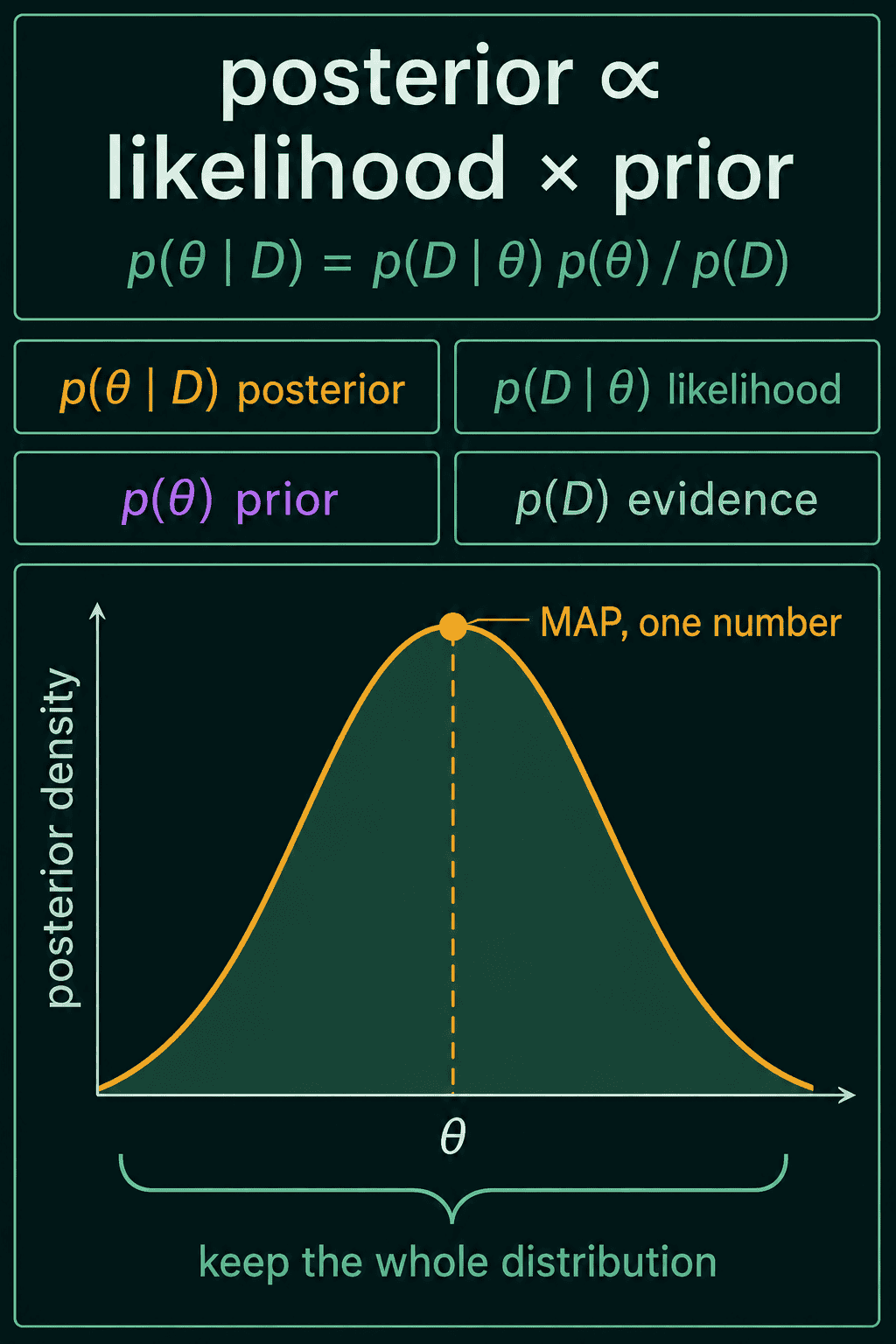
Write the unknown parameter as $\theta$ (theta) and the observed data as $D$. For the coin, $\theta$ is the probability of heads and $D$ is the list of 10 flips. Bayes' theorem uses four quantities:

The prior $p(\theta)$ is the belief about $\theta$ before any data, written as a probability distribution.
The likelihood $p(D \mid \theta)$ is the probability of the observed data if the parameter were $\theta$. The vertical bar reads "given".
The posterior $p(\theta \mid D)$ is the belief about $\theta$ after seeing the data.
The evidence $p(D)$ is the overall probability of the data, averaged over every possible $\theta$.

The formula is

$$p(\theta \mid D)=\frac{p(D \mid \theta)\,p(\theta)}{p(D)}$$

The posterior is the likelihood times the prior, divided by the evidence so that it adds up to 1. The evidence is the same number for every $\theta$, so the rule is often written as posterior $\propto$ likelihood $\times$ prior. The symbol $\propto$ means "proportional to": equal up to a constant.

For the coin, take a flat prior: every value of $\theta$ between 0 and 1 starts out equally plausible. The likelihood of 7 heads and 3 tails is $\theta^7(1-\theta)^3$, one factor of $\theta$ per head and one factor of $1-\theta$ per tail. At $\theta = 0.5$ it is $0.5^{10} \approx 0.00098$, and at $\theta = 0.7$ it is about $0.0022$. With a flat prior the posterior has the same shape as the likelihood, so after these flips 0.7 is about 2.3 times as plausible as 0.5.

Computing the evidence

The evidence adds up the likelihood times the prior over every possible parameter value:

$$p(D)=\int p(D \mid \theta)\,p(\theta)\,d\theta$$

If $\theta$ can take only a few values, the integral is a plain sum. With one parameter it can be approximated on a grid of candidate values. Most models have far too many parameters for a grid, and for most of them the integral has no closed form either.

For the coin a grid of 999 values works fine. Score each candidate with likelihood times prior, then divide by the total so the scores add up to 1:

1import torch
2 
3p = torch.linspace(0.001, 0.999, 999)       # candidate values of the probability of heads
4prior = torch.ones_like(p)                  # flat prior
5likelihood = p**7 * (1 - p)**3              # 7 heads, 3 tails
6unnormalized = likelihood * prior
7posterior = unnormalized / unnormalized.sum()   # the sum plays the role of p(D)
8 
9print(round(p[posterior.argmax()].item(), 3))   # peak of the posterior
10print(round((p * posterior).sum().item(), 3))   # posterior mean
11# 0.7
12# 0.667

The peak of the posterior is the maximum a posteriori (MAP) estimate. MAP can skip the evidence entirely, because $p(D)$ does not depend on $\theta$ and so cannot move the peak. With a flat prior the peak lands at 0.7, the same as the MLE. The posterior mean, each candidate weighted by its posterior probability, is 0.667. Bayesian inference keeps the whole curve rather than one point on it:

A posterior density curve over theta with its peak marked as MAP, one number, and a bracket under the whole curve saying keep the whole distribution, above Bayes' theorem written as posterior proportional to likelihood times prior and four labels for the posterior, likelihood, prior and evidence.

Credible intervals

With the full posterior, questions about uncertainty become sums over the grid. A credible interval is a range that holds the parameter with a stated posterior probability. The central 95% one runs from the point with 2.5% of the posterior below it to the point with 97.5% below it:

1import torch
2 
3p = torch.linspace(0.001, 0.999, 999)
4posterior = p**7 * (1 - p)**3
5posterior = posterior / posterior.sum()
6cdf = posterior.cumsum(0)                       # posterior probability below each candidate
7low = p[(cdf >= 0.025).nonzero()[0]].item()
8high = p[(cdf >= 0.975).nonzero()[0]].item()
9print(round(low, 2), round(high, 2))
10print(round(posterior[p >= 0.5].sum().item(), 3))   # probability that heads is favored
11# 0.39 0.89
12# 0.887

After 10 flips the probability of heads lies between 0.39 and 0.89 with 95% probability, and there is an 89% chance the coin favors heads. A credible interval is the Bayesian counterpart of a confidence interval, read straight off the posterior.

The posterior also shows when two different parameter settings both explain the data well. A point estimate picks one of them and hides the other. That is the motivation behind Bayesian neural networks and other models that need to say how unsure they are.

Conjugate priors

The grid gets expensive fast, so some prior and likelihood pairs are chosen because the posterior comes out in closed form. A prior is conjugate to a likelihood when the posterior belongs to the same family of distributions as the prior.

A common example is a coin. A single flip is a Bernoulli variable: 1 (heads) with probability $\theta$ and 0 (tails) otherwise. A natural prior for $\theta$ is the Beta distribution, which lives on exactly the range 0 to 1. A Beta with parameters $\alpha$ (alpha) and $\beta$ (beta) has density and mean

$$p(x) \propto x^{\alpha-1}(1-x)^{\beta-1}$$

$$E[X] = \frac{\alpha}{\alpha+\beta}$$

$\mathrm{Beta}(1, 1)$ has density $x^0(1-x)^0 = 1$, the flat prior used above.

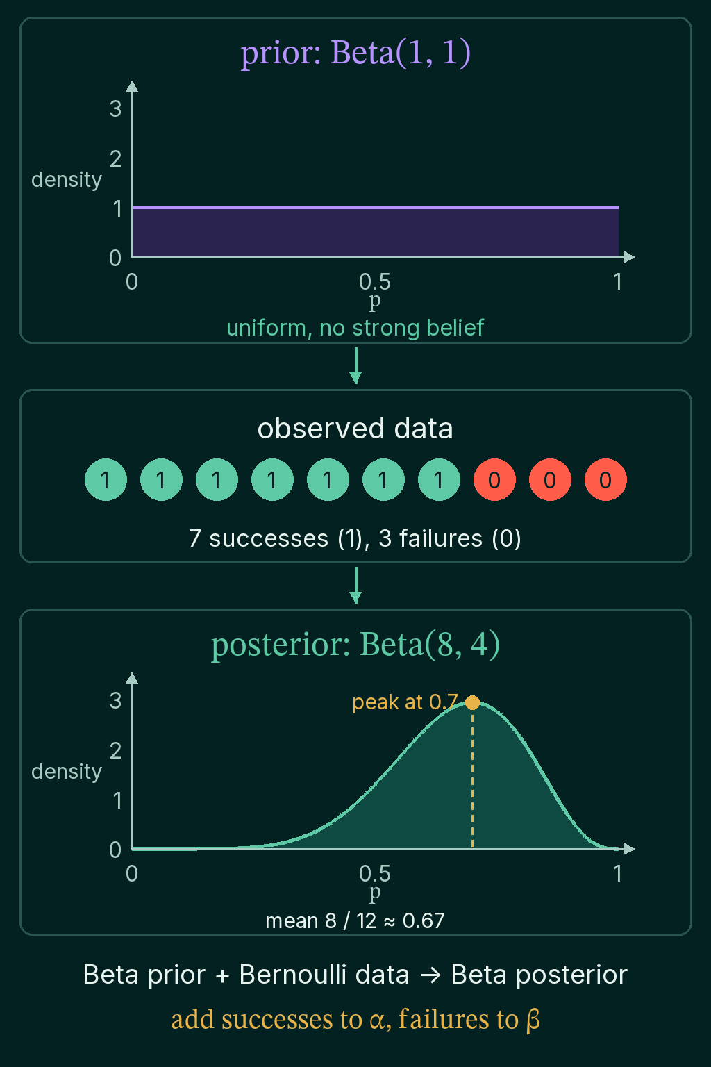
Multiply the likelihood $\theta^7(1-\theta)^3$ by the flat prior and the result is $\theta^7(1-\theta)^3$, which is the shape of $\mathrm{Beta}(8, 4)$ because the exponents are $\alpha - 1$ and $\beta - 1$. In general, a $\mathrm{Beta}(\alpha, \beta)$ prior followed by $s$ successes and $f$ failures gives

$$\mathrm{Beta}(\alpha+s,\ \beta+f)$$

Add the successes to $\alpha$ and the failures to $\beta$. That is why $\alpha$ and $\beta$ are often read as pseudo-counts, heads and tails the prior counts as already seen. The posterior mean of $\mathrm{Beta}(8, 4)$ is $8/12 \approx 0.667$, the same value the grid found:

1from torch.distributions import Beta
2 
3alpha, beta = 1.0, 1.0               # prior Beta(1, 1)
4heads, tails = 7, 3
5post = Beta(alpha + heads, beta + tails)
6print(post.concentration1.item(), post.concentration0.item())   # alpha and beta of the posterior
7print(round(post.mean.item(), 4))
8# 8.0 4.0
9# 0.6667

The posterior mean 0.667 sits a little below the MLE of 0.7, pulled toward the prior's one pseudo-head and one pseudo-tail. The update needs only addition, with no grid and no sampling:

A flat Beta(1, 1) prior over p, then 7 successes and 3 failures, then the Beta(8, 4) posterior curve peaking at 0.7 with mean 0.67, with the rule Beta prior plus Bernoulli data gives a Beta posterior, add successes to alpha and failures to beta.

The posterior predictive distribution

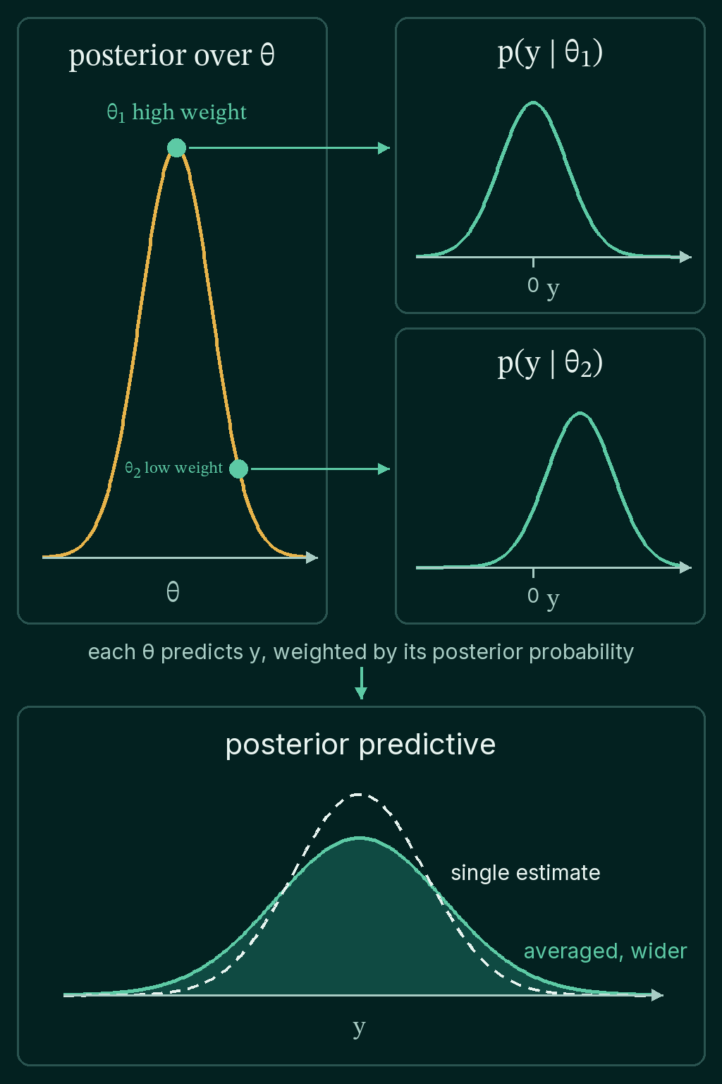
A posterior describes the parameter, while most of the time the question is about the next observation. The posterior predictive distribution answers it by averaging the prediction of every parameter value, weighted by how plausible that value is:

$$p(y_{new} \mid D)=\int p(y_{new} \mid \theta)\,p(\theta \mid D)\,d\theta$$

$p(y_{new} \mid \theta)$ is the prediction a single value $\theta$ makes for a new observation $y_{new}$, and $p(\theta \mid D)$ is the weight it gets. With samples drawn from the posterior, the integral becomes a plain average over those samples.

For the coin, $\theta$ samples come from $\mathrm{Beta}(8, 4)$. A Binomial(10, $\theta$) count is the number of heads in 10 flips when each flip lands heads with probability $\theta$. The code compares plugging in the single value 0.7 against averaging over the posterior:

1import torch
2from torch.distributions import Beta, Binomial
3 
4torch.manual_seed(0)
5theta = Beta(8.0, 4.0).sample((100_000,))         # samples from the posterior
6 
7print(round(theta.mean().item(), 3))              # probability the next flip is heads
8 
9plug_in = Binomial(10, probs=torch.tensor(0.7)).sample((100_000,))
10predictive = Binomial(10, probs=theta).sample()   # one draw per posterior sample
11print(round(plug_in.var().item(), 2), round(predictive.var().item(), 2))
12print(round((plug_in <= 4).float().mean().item(), 3), round((predictive <= 4).float().mean().item(), 3))
13# 0.667
14# 2.11 3.74
15# 0.048 0.14

The probability that the next flip lands heads is 0.667. For the next 10 flips, the plug-in prediction has a variance of 2.11 and the posterior predictive has a variance of 3.74. The plug-in gives only a 4.8% chance of 4 heads or fewer, because it assumes the coin is exactly 0.7. The posterior predictive gives 14%, because it still counts the chance that the coin is close to fair. A prediction interval read from it is wider for the same reason:

A posterior over theta with a high-weight value theta 1 and a low-weight value theta 2, each with its own prediction curve over y, combined by a weighted average into a posterior predictive curve that is wider than the dashed single-estimate curve.

When to use it, and common mistakes

Bayesian inference is worth the extra compute when data is scarce, when a prior belief is worth encoding, or when the downstream decision needs to know how unsure the model is. With a lot of data the posterior narrows around the MLE, and a point estimate gives nearly the same predictions for far less compute.

Treating MAP as Bayesian inference. MAP keeps only the peak of the posterior and throws away its width.
Plugging one estimate into a prediction. The plug-in prediction above is too confident, with a variance of 2.11 instead of 3.74.
Running a grid over many parameters. 1,000 values per parameter is $1000^{10}$ grid points for 10 parameters, which is why sampling methods exist.
Forgetting the prior. With 10 flips, $\mathrm{Beta}(1, 1)$ and $\mathrm{Beta}(50, 50)$ give very different posteriors, so the prior is part of the result and worth reporting.

Bayes' theorem covers the formula itself with a spam-filter example. MLE vs MAP estimation covers the two point estimates and how a prior turns into regularization. The common probability distributions post introduces the Beta distribution in more detail. Monte Carlo methods explains how to average over samples when the posterior has no closed form.

QuiddityML teaches Bayesian inference, the posterior predictive distribution and conjugate priors as three concepts in the Math track's probability unit, and the exercises on them include normalizing a posterior over a grid and implementing beta_bernoulli_mean to update a Beta prior from a list of outcomes.