By Sagi Shaier · 19 October 2026 · 7 min read

Monte Carlo methods explained: Monte Carlo estimation, importance sampling, and rejection sampling

What error to expect from an average of random samples, and how importance sampling and rejection sampling handle targets that are hard to sample from. The PyTorch examples also show why both struggle in high dimensions.

Monte Carlo methods estimate a quantity by drawing random samples and averaging something over them. They are the usual fallback when an expectation or a probability is too hard to compute exactly. A common case in machine learning is an integral over every parameter value, like the one in the denominator of Bayes' theorem.

Monte Carlo estimation

The expected value $\mathbb{E}[f(X)]$ is the average value a function $f$ takes when its input $X$ is drawn from some distribution. Computing it exactly means an integral over every possible value of $X$. Monte Carlo estimation replaces the integral with an average over $n$ samples $x_1, \dots, x_n$ drawn from the distribution of $X$:

$$\mathbb{E}[f(X)] \approx \frac{1}{n}\sum_{i=1}^{n} f(x_i)$$

To check the method, take a case with a known answer. If $X$ follows a standard normal distribution with mean 0 and variance 1, then $\mathbb{E}[X^2]$ is exactly its variance of 1. Draw samples, square them and average:

1import torch
2 
3torch.manual_seed(0)
4for n in (100, 400, 1_600, 6_400):
5    x = torch.randn(n)                    # samples of X from a standard normal
6    f = x**2                              # f(X) = X squared, true expectation 1
7    estimate = f.mean()
8    std_error = f.std() / n**0.5
9    print(f"n={n:5d}  estimate {estimate:.3f}  standard error {std_error:.3f}")
10# n=  100  estimate 1.051  standard error 0.170
11# n=  400  estimate 0.946  standard error 0.063
12# n= 1600  estimate 1.030  standard error 0.037
13# n= 6400  estimate 0.985  standard error 0.017

How accurate is a Monte Carlo estimate?

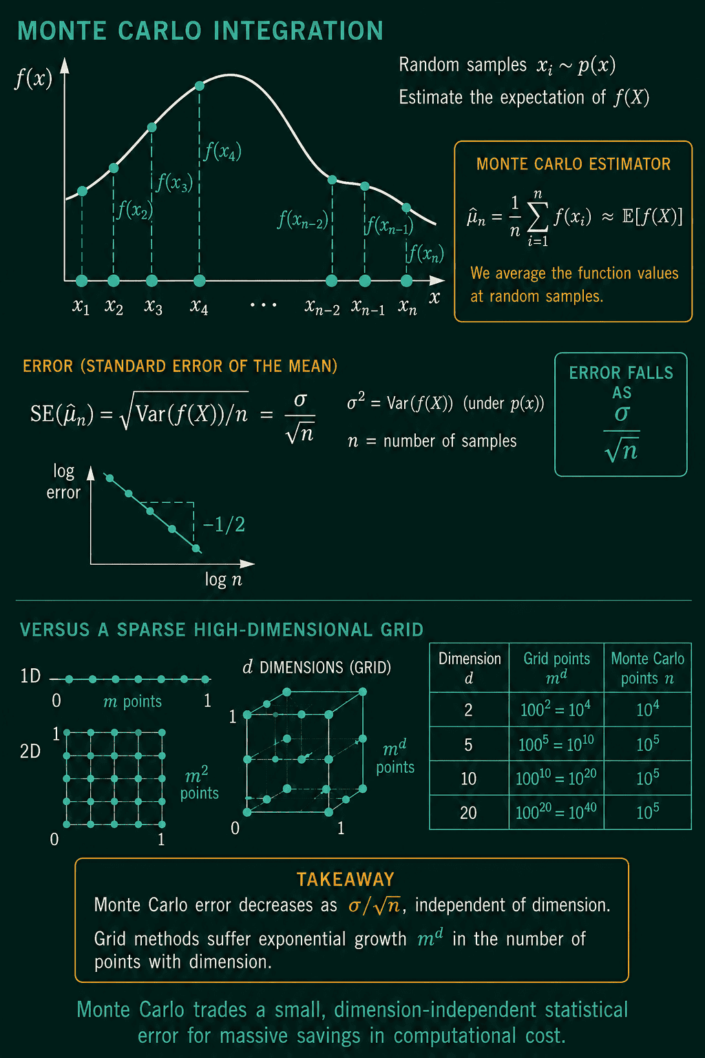
The Monte Carlo estimate is a sample mean, so its typical error is the standard error of a mean, $\sigma/\sqrt{n}$. Here $\sigma$ is the standard deviation of $f(X)$ and $n$ is the number of samples. Four times as many samples halve the error. In the run above the sample count grows 64 times from 100 to 6,400. The standard error falls from 0.170 to 0.017, close to the factor of 8 that $\sqrt{64}$ predicts.

The formula has no term for the number of dimensions. A grid that puts 100 points along each axis needs $100^{10} = 10^{20}$ points in 10 dimensions, while the Monte Carlo error depends only on $\sigma$ and $n$. That is why random samples can still give a usable estimate in problems with many dimensions:

A curve f(x) evaluated at random sample points x1 to xn, the Monte Carlo estimator as the average of the f values, the standard error sigma over the square root of n with a log-log plot of slope minus one half, and a comparison of grid points m to the d against Monte Carlo sample counts for 2 to 20 dimensions.

Importance sampling

Plain Monte Carlo struggles when the samples that count are rare. Take the probability that a standard normal value lands above 3, about 0.00135. Write it as an expectation: $f(x)$ is 1 when $x > 3$ and 0 otherwise. Out of 10,000 samples only a handful land above 3, so the estimate rests on those few.

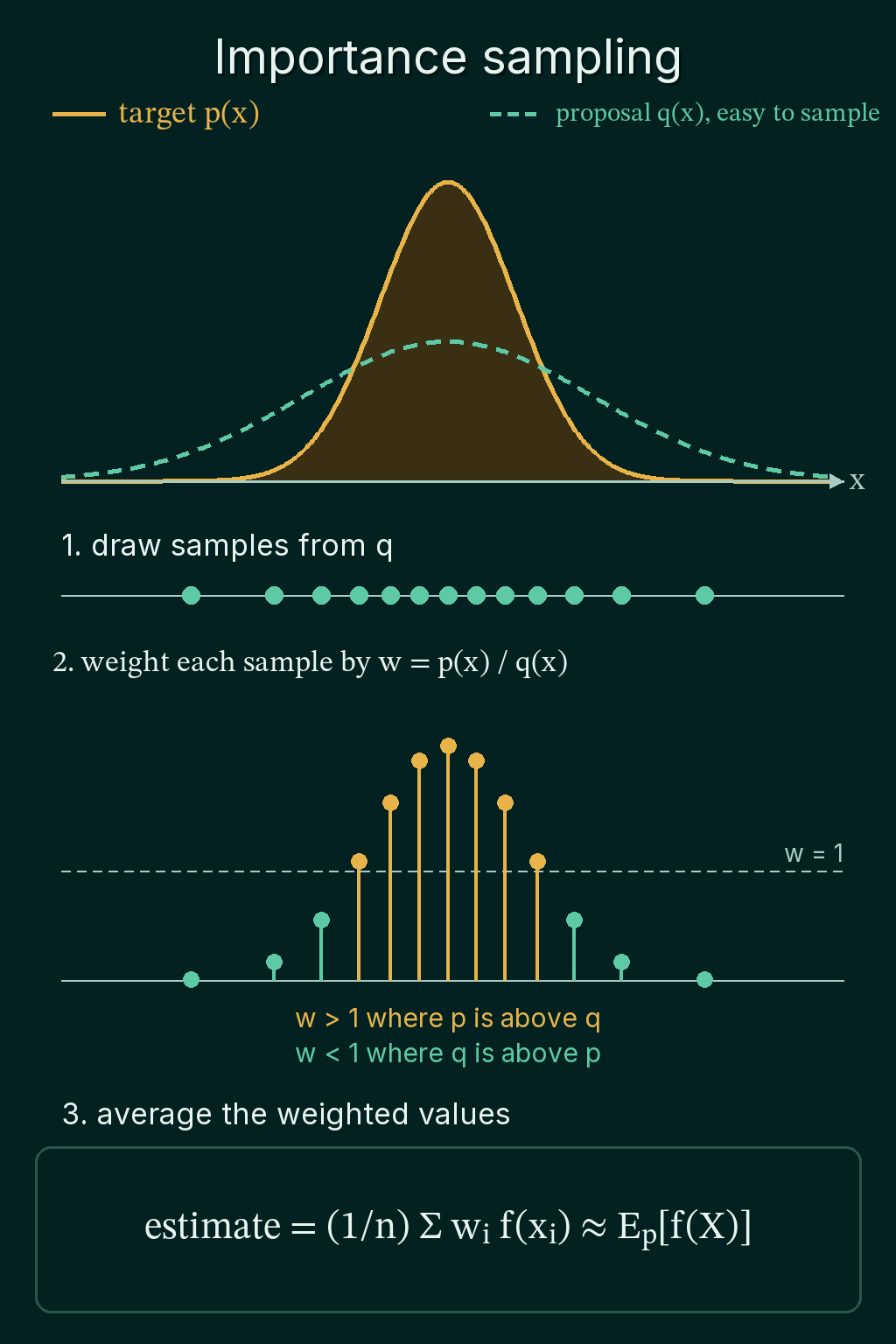
Importance sampling draws the samples from an easier distribution $q(x)$ called the proposal, then corrects for that with a weight. The distribution the expectation is actually about, $p(x)$, is called the target. Each sample gets the weight

$$w_i = \frac{p(x_i)}{q(x_i)}$$

and the estimate becomes a weighted average:

$$\mathbb{E}_p[f(X)] \approx \frac{1}{n}\sum_{i=1}^n w_i\, f(x_i)$$

A sample that $q$ produces more often than $p$ would gets a weight below 1, and a sample that $q$ produces less often gets a weight above 1. Every draw is kept. Here the proposal is a normal distribution centered at 3.5, so about two thirds of its samples land above 3:

1import torch
2from torch.distributions import Normal
3 
4torch.manual_seed(0)
5p = Normal(0.0, 1.0)                      # target
6n = 10_000
7 
8x = p.sample((n,))
9print((x > 3).sum().item(), round((x > 3).float().mean().item(), 5))   # plain Monte Carlo
10 
11q = Normal(3.5, 1.0)                      # proposal centered on the tail
12x = q.sample((n,))
13w = (p.log_prob(x) - q.log_prob(x)).exp() # importance weights p(x) / q(x)
14print(round((w * (x > 3)).mean().item(), 5))
15print(round((1 - p.cdf(torch.tensor(3.0))).item(), 5))                 # exact answer
16# 18 0.0018
17# 0.00138
18# 0.00135

Plain Monte Carlo saw 18 samples above 3 and answered 0.0018, a third too high. Importance sampling answered 0.00138, against the exact 0.00135. The weights are computed as a difference of log-probabilities and then exponentiated, because the raw densities far out in the tail are tiny numbers that lose precision.

A narrow target density p of x and a wider dashed proposal q of x, samples drawn from q, a weight w equal to p over q for each sample that is above 1 near the center where p is above q and below 1 in the tails, and the reweighted average as the importance sampling estimate.

Self-normalized importance sampling

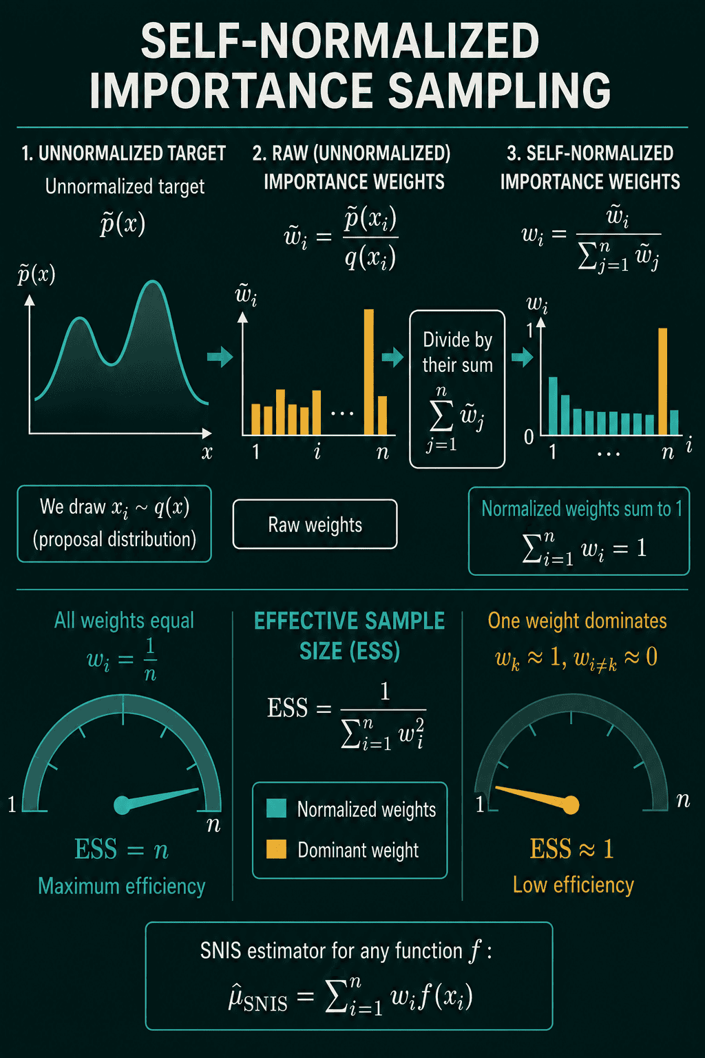
The weights above need $p(x)$ exactly. Often only an unnormalized version $\tilde p(x)$ is available: the right shape, but missing the constant that makes it integrate to 1. A posterior is a common example, since its normalizing constant is the hard integral itself. Self-normalized importance sampling divides each weight by the sum of all the weights:

$$\mathbb{E}[f(X)] \approx \sum_{i=1}^n \frac{\tilde w_i}{\sum_j \tilde w_j}\, f(x_i)$$

$$\tilde w_i = \frac{\tilde p(x_i)}{q(x_i)}$$

The missing constant multiplies every weight by the same amount, so it cancels in the division without ever being computed. The price is a small bias, because one random sum is divided by another. That bias shrinks like $1/n$, and in exchange the estimate often has much lower variance.

Effective sample size

Importance sampling can fail quietly when most of the weight lands on a few draws. The average then really comes from those few points while it looks like it used all of them. The effective sample size says how many samples the estimate behaves as if it used:

$$n_{\text{eff}} = \frac{(\sum_i w_i)^2}{\sum_i w_i^2}$$

Equal weights give $n$, and one weight carrying everything gives 1. The code estimates $\mathbb{E}[X^2] = 1$ for a standard normal known only up to its constant $1/\sqrt{2\pi}$, once with a wide proposal centered on the target and once with a proposal centered at 3.5:

1import torch
2from torch.distributions import Normal
3 
4torch.manual_seed(0)
5for q in (Normal(0.0, 2.0), Normal(3.5, 1.0)):
6    x = q.sample((10_000,))
7    p_tilde = torch.exp(-x**2 / 2)            # standard normal without its 1 / sqrt(2 pi)
8    w = p_tilde / q.log_prob(x).exp()         # unnormalized weights
9    w_norm = w / w.sum()                      # self-normalized weights
10    estimate = (w_norm * x**2).sum()          # E[X^2], true value 1
11    ess = w.sum() ** 2 / (w ** 2).sum()       # effective sample size
12    print(f"q mean {q.mean.item():.1f}  estimate {estimate:.3f}  ESS {ess:.0f}")
13# q mean 0.0  estimate 1.001  ESS 6608
14# q mean 3.5  estimate 0.578  ESS 12

The wide proposal gives 1.001 with an effective sample size of 6,608 out of 10,000. The proposal at 3.5 rarely lands where the target has its mass, so a dozen draws near the center carry nearly all the weight. Its 10,000 samples behave like 12, and the estimate of 0.578 is far from 1:

Self-normalized importance sampling in three steps, an unnormalized target, raw weights, and weights divided by their sum, then the effective sample size formula with a gauge at n when all weights are equal and a gauge near 1 when one weight dominates.

Rejection sampling

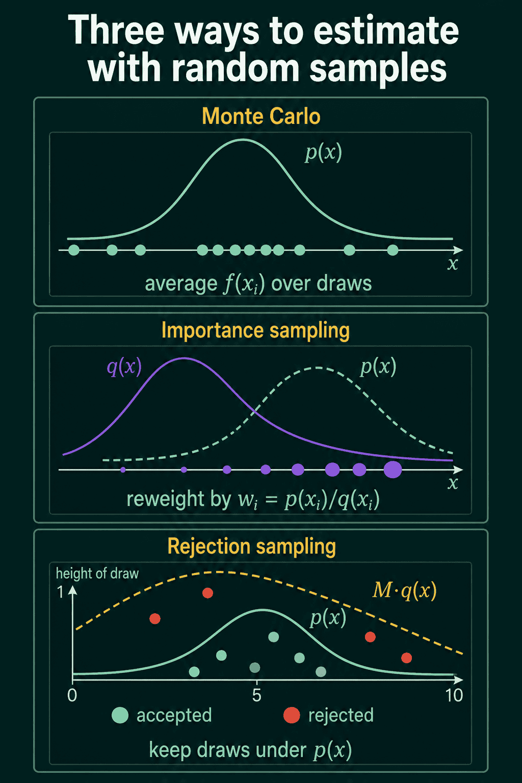
Rejection sampling also draws from a proposal $q(x)$, but instead of reweighting it throws samples away, and the samples it keeps are distributed exactly like the target $p$. It needs a constant $M$ such that the envelope $M \cdot q(x)$ stays at or above $p(x)$ everywhere. For each draw $x_i$ from $q$, also draw $u_i$ uniformly between 0 and 1, and keep $x_i$ only if

$$u_i \le \frac{p(x_i)}{M \cdot q(x_i)}$$

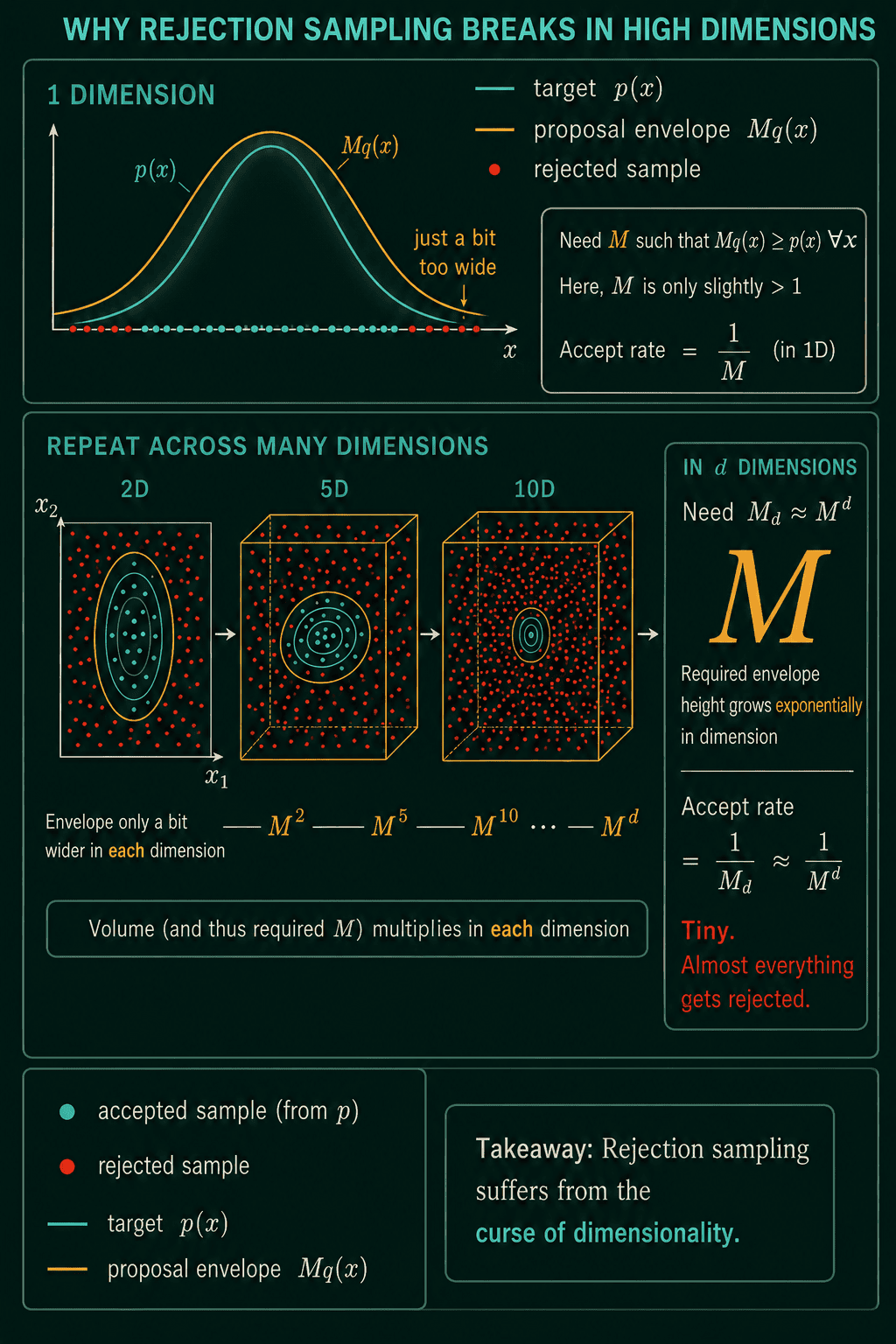
Geometrically, the rule places the draw at height $u_i \cdot M \cdot q(x_i)$ under the envelope, and keeps it if that point is also under $p(x)$. When $p$ and $q$ are both normalized, the fraction of draws kept is exactly $1/M$. Every rejected draw is wasted work, so the smallest $M$ that still keeps the envelope above $p$ is the one to use:

Three panels: Monte Carlo averaging f over draws from p, importance sampling with a proposal q and a target p and sample dots sized by their weights, and rejection sampling with draws under an envelope M times q of x, kept when they fall under p of x and rejected otherwise.

Rejection sampling in high dimensions

The envelope has to cover the target in every direction at once. Take a standard normal target and a proposal that is a normal 1.1 times too wide. The ratio $p/q$ is largest at the center, where it is 1.1 per dimension, so in $d$ dimensions the smallest envelope is $M = 1.1^d$:

1import torch
2 
3torch.manual_seed(0)
4n = 100_000
5log_2pi = torch.log(torch.tensor(2 * torch.pi))
6for d in (1, 10, 50):
7    M = 1.1 ** d                                   # smallest envelope for this pair
8    x = 1.1 * torch.randn(n, d)                    # proposal: a normal 1.1 times too wide
9    log_p = -(x**2).sum(1) / 2 - d * 0.5 * log_2pi
10    log_q = -(x**2).sum(1) / (2 * 1.1**2) - d * (0.5 * log_2pi + torch.log(torch.tensor(1.1)))
11    u = torch.rand(n)
12    accept = u <= (log_p - log_q).exp() / M
13    print(f"d={d:3d}  M={M:8.1f}  accepted {accept.float().mean():.4f}  1/M {1/M:.4f}")
14print(round(1.1 ** 100))
15# d=  1  M=     1.1  accepted 0.9093  1/M 0.9091
16# d= 10  M=     2.6  accepted 0.3870  1/M 0.3855
17# d= 50  M=   117.4  accepted 0.0080  1/M 0.0085
18# 13781

In one dimension 91% of draws survive. In 50 dimensions it is under 1%. In 100 dimensions $M \approx 13{,}781$, so about one draw in 14,000 is kept. Importance sampling degrades the same way, through a shrinking effective sample size instead of a shrinking accept rate:

Rejection sampling in one dimension with an envelope only slightly wider than the target, then the same slack compounding across 2, 5 and 10 dimensions so the required envelope grows like M to the d and the accept rate 1 over M to the d becomes tiny.

Which one to use, and common mistakes

Plain Monte Carlo is the default whenever the target can be sampled directly. Importance sampling fits when the samples that count are rare under the target, or when the target can be evaluated but not sampled. Rejection sampling fits when exact samples are needed and the problem has only a few dimensions. Both of the last two degrade on targets with many dimensions, where a different family of methods called Markov chain Monte Carlo is the usual choice.

Reporting $n$ instead of the effective sample size. 10,000 importance samples with an effective sample size of 12 carry the information of about 12 draws.
Computing weights from raw densities. Far in the tail $p(x)$ and $q(x)$ are tiny, so subtract log-probabilities and exponentiate at the end.
An envelope that dips below the target. If $M \cdot q(x) < p(x)$ anywhere, the kept samples no longer follow $p$.
A proposal narrower than the target. The tails of $p$ then get almost no draws, and a few huge weights dominate the estimate.

The law of large numbers and the central limit theorem explain why an average of samples settles on the expectation. Standard error and confidence intervals cover the $\sigma/\sqrt{n}$ error in detail. Bayesian inference is a common place these methods get used, because the posterior's normalizing constant is often an intractable integral. The curse of dimensionality post covers the same high-dimensional effect from the data side.

QuiddityML teaches Monte Carlo estimation, importance sampling and rejection sampling as three concepts in the Math track's probability unit, and the exercises on them include implementing monte_carlo_estimate and picking the rule that decides when rejection sampling keeps a draw.