By Sagi Shaier · 8 October 2026 · 5 min read

Multicollinearity explained: why correlated features break linear regression

Multicollinearity is when two or more features in a dataset carry almost the same information. This post explains why that makes a linear model's weights unstable even when its predictions look fine, shows it happening in PyTorch, and covers what to do about it.

Collinearity is when two features in a dataset are almost exact copies of each other up to scaling, and multicollinearity is the same thing spread across more than two features. It shows up in real data all the time, for example a height column recorded in inches next to the same height in centimeters. A model trained on features like these can still predict well, but the weights it learns for those features stop meaning anything, and they can change wildly from one training run to the next.

Exact dependence and near dependence

Treat each feature column of a dataset as a vector, with one entry per row. A set of vectors is linearly dependent when one of them can be built exactly by scaling and adding the others. If a price_in_dollars column were always exactly 1.1 times a price_in_euros column, the dollar column would be linearly dependent on the euro column and would add no information.

Real data is rarely that tidy. Measurements carry rounding and noise, so two columns that describe the same thing end up nearly dependent instead of exactly dependent. Collinearity is that near dependence: two or more feature vectors that are close to linearly dependent without being exactly so.

Take a dataset with a height_in_inches column and a height_in_cm column. The centimeter value is roughly 2.54 times the inch value, and across every row that ratio barely moves. The two columns hold almost the same information twice.

Why near-duplicate features make weights unstable

A linear model predicts by multiplying each feature by a weight and adding the results. With the two height features, a prediction looks like

$$\hat{y} = w_{\text{in}} \cdot x_{\text{in}} + w_{\text{cm}} \cdot x_{\text{cm}} + b$$

where $x_{\text{in}}$ and $x_{\text{cm}}$ are the two height values for one row, $w_{\text{in}}$ and $w_{\text{cm}}$ are their weights, $b$ is a constant offset called the intercept, and $\hat{y}$ is the prediction.

Since $x_{\text{cm}}$ is close to $2.54 \cdot x_{\text{in}}$ on every row, the two weighted terms do almost the same job. Raise $w_{\text{in}}$ by 2.54 and lower $w_{\text{cm}}$ by 1, and the prediction barely changes, because the extra $2.54 \cdot x_{\text{in}}$ is cancelled by the missing $x_{\text{cm}}$. The weights $(1, 0)$, $(-1.54, 1)$ and $(3.54, -1)$ all give the same prediction, and so does every other pair on that line.

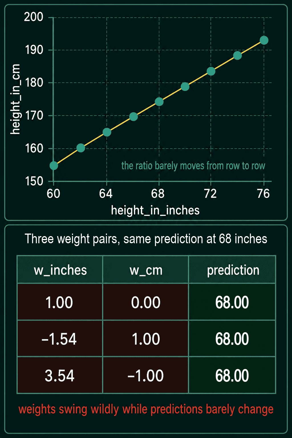
A scatter of height in centimeters against height in inches lying almost on a straight line, and a table of three very different weight pairs, (1.00, 0.00), (minus 1.54, 1.00) and (3.54, minus 1.00), that all give the same prediction

Training has to pick one pair, and with many pairs scoring almost the same, which one it picks depends on small details of the training data. Remove a few rows or add a little noise and the chosen weights can jump a long way while the predictions hardly move. That makes the weights unreliable to read: a large positive weight on one height column and a negative weight on the other says nothing about how height relates to the target.

Seeing it in PyTorch

The snippet below builds 50 people with a height in inches, a height in centimeters that is 2.54 times the inches plus a little measurement noise, and a body weight that depends on height. It fits a linear model three times, each time on a different random resample of the 50 rows, and prints the learned weights and the prediction for a new person who is 70 inches tall.

1import torch
2 
3torch.manual_seed(0)
4n = 50
5inches = 60 + 16 * torch.rand(n)
6cm = 2.54 * inches + 0.5 * torch.randn(n)    # nearly 2.54 * inches, plus measurement noise
7weight_kg = 1.2 * inches - 10 + 3 * torch.randn(n)   # the target
8 
9print(torch.corrcoef(torch.stack([inches, cm])))
10 
11X = torch.stack([inches, cm, torch.ones(n)], dim=1)   # two features plus an intercept column
12new_person = torch.tensor([[70.0, 177.8, 1.0]])
13 
14for trial in range(3):
15    idx = torch.randint(0, n, (n,))                  # resample the 50 rows with replacement
16    w = torch.linalg.lstsq(X[idx], weight_kg[idx].unsqueeze(1)).solution.squeeze()
17    pred = (new_person @ w).item()
18    print(f"w_inches={w[0].item():7.2f}  w_cm={w[1].item():6.2f}  prediction={pred:.1f}")
19 
20X1 = torch.stack([inches, torch.ones(n)], dim=1)     # inches only, plus the intercept
21for trial in range(3):
22    idx = torch.randint(0, n, (n,))
23    w = torch.linalg.lstsq(X1[idx], weight_kg[idx].unsqueeze(1)).solution.squeeze()
24    pred = (new_person[:, [0, 2]] @ w).item()
25    print(f"w_inches={w[0].item():5.2f}  prediction={pred:.1f}")

1tensor([[1.0000, 0.9989],
2        [0.9989, 1.0000]])
3w_inches=   4.00  w_cm= -1.18  prediction=73.7
4w_inches=   6.34  w_cm= -1.97  prediction=73.9
5w_inches=   6.64  w_cm= -2.16  prediction=74.5
6w_inches= 1.16  prediction=73.8
7w_inches= 1.25  prediction=74.3
8w_inches= 1.08  prediction=74.0

torch.corrcoef gives the correlation between the two columns, 0.9989, where 1 would mean they lie on a perfect straight line. torch.linalg.lstsq finds the weights that minimize the squared error of a linear model. With both height columns, the inch weight moves from 4.00 to 6.64 across resamples and the centimeter weight turns negative, while the prediction stays between 73.7 and 74.5 kg. With the inch column alone, the weight stays between 1.08 and 1.25, close to the 1.2 used to make the data, and the predictions land in the same range as before.

What to do about it

A first check is to look for pairs of columns that move together almost perfectly. A correlation near 1 or -1 between two features, like the 0.9989 above, is a warning sign worth acting on rather than a coincidence.

When two columns measure the same thing, dropping one is usually the simplest fix, as the inches-only fit shows. Two broader tools help when the overlap is spread across many features. Regularization adds a penalty for large weights to the training loss, which keeps any one weight from swinging far in one direction while its partner swings the other way. Dimensionality reduction rewrites the feature set as a smaller set of independent directions, which removes the redundancy before the model sees it.

Common mistakes

Reading weights as importance when features overlap. A negative weight on height_in_cm next to a large positive weight on height_in_inches says nothing about the effect of height.
Judging the model only by its predictions. Predictions can look stable while the weights underneath are not, so a model that predicts well can still give misleading weights.
Expecting exact dependence before worrying. Columns do not need to be exact multiples of each other, and a correlation of 0.99 is enough to make weights swing.
Checking only pairs. Three or more features can be nearly dependent together even when no single pair looks alarming, which is the "multi" in multicollinearity.

Linear independence is the exact version of this idea, where no feature can be built from the others at all, covered in span, basis and linear independence. Vectors and matrices, including how a dataset becomes a matrix of feature columns, are in vectors and matrices for machine learning.

QuiddityML teaches collinearity as its own concept in the linear algebra part of the Math track, and the exercises on it include spotting which feature pairs are collinear, ordering the lines of an is_collinear check on two feature columns, and writing that check from scratch.