By Sagi Shaier · 18 October 2026 · 7 min read
Standard error and confidence intervals explained
How to put an error bar on an average, such as a validation accuracy or a mean latency, how to compute it by hand and in PyTorch, and what 95% confidence does and does not promise.
The standard error of an average is how much that average would change if you collected a fresh sample of the same size and computed it again. A confidence interval turns the standard error into a range around the average, such as "accuracy 0.87, between 0.85 and 0.89". Any number computed from a sample comes with this kind of uncertainty, from a validation accuracy to an average response time. The standard error is the usual way to report how large it is.
Averages move from sample to sample
Suppose the true average response time of a service is 120 ms. Measure 40 requests and the average might come out at 117 ms. Measure another 40 and it might be 124 ms. The average you compute depends on which requests happened to land in your sample.
The spread of those repeated averages has a simple formula. If single measurements have standard deviation $\sigma$ (sigma), the average of $n$ independent measurements has spread
$$\mathrm{SE}(\bar{X}) = \frac{\sigma}{\sqrt{n}}$$
$\bar{X}$ (read "X bar") is the sample average, and $\mathrm{SE}$ stands for standard error. The square root is why more data helps slowly: four times the data halves the standard error. Here are standard errors from samples of a distribution with $\sigma = 1$:
1import torch
2
3torch.manual_seed(0)
4for n in (100, 400, 1_600):
5    x = torch.randn(n)
6    print(n, round((x.std() / n ** 0.5).item(), 4))
7# 100 0.103
8# 400 0.0487
9# 1600 0.0254
Each step multiplies the sample size by 4, and the standard error drops by about half each time.
Estimating the spread from the data
The formula needs $\sigma$, the spread of single measurements, and in practice you rarely know it. You estimate it from the same data with the sample standard deviation $s$:
$$s = \sqrt{\frac{1}{n-1}\sum_{i=1}^n (x_i - \bar{x})^2}$$
In words: subtract the average from every value and square the differences. Then add them up, divide by $n-1$ and take the square root. The divisor is $n-1$ rather than $n$ because the average $\bar{x}$ was itself computed from the same data, which uses up one degree of freedom: once you know the average and $n-1$ of the differences, the last difference is fixed.
Take five measurements: 4, 7, 6, 3 and 5. Their average is $\bar{x} = 25/5 = 5$. The differences from 5 are $-1, 2, 1, -2, 0$, and their squares are $1, 4, 1, 4, 0$, which add up to 10. Dividing by $n - 1 = 4$ gives 2.5, so $s = \sqrt{2.5} = 1.581$.
Putting $s$ in place of $\sigma$ gives the estimated standard error:
$$\widehat{\mathrm{SE}}(\bar{X}) = \frac{s}{\sqrt{n}}$$
The hat marks an estimate. For the five measurements it is $1.581 / \sqrt{5} = 0.707$.
A 95% confidence interval
A rough 95% confidence interval for the mean is the average plus or minus 1.96 standard errors:
$$\bar{x} \pm 1.96\,\widehat{\mathrm{SE}}(\bar{X})$$
The 1.96 comes from the standard Gaussian, the bell curve with mean 0 and standard deviation 1. 95% of its probability lies between $-1.96$ and $1.96$, with 2.5% above and 2.5% below. In the language of quantiles, 1.96 is the 0.975 quantile of the standard Gaussian: the value with 97.5% of the probability below it. A different multiplier gives a different confidence level, 1.645 for 90% and 2.576 for 99%.
For the five measurements, the interval is $5 \pm 1.96 \times 0.707$, which runs from 3.61 to 6.39.
In PyTorch, x.std() computes $s$ with the $n-1$ divisor and x.numel() counts the values, so the whole calculation is three lines:
1import torch
2
3x = torch.tensor([4.0, 7.0, 6.0, 3.0, 5.0])
4n = x.numel()
5mean = x.mean()
6s = x.std()                 # divides by n - 1
7se = s / n ** 0.5
8
9print(round(mean.item(), 3), round(s.item(), 3), round(se.item(), 3))
10print("1.96: ", round((mean - 1.96 * se).item(), 2), round((mean + 1.96 * se).item(), 2))
11print("2.776:", round((mean - 2.776 * se).item(), 2), round((mean + 2.776 * se).item(), 2))
12# 5.0 1.581 0.707
13# 1.96:  3.61 6.39
14# 2.776: 3.04 6.96
The last line uses a wider multiplier, and the next section explains why five values call for it.
When 1.96 is too narrow
The 1.96 multiplier is exact when $\sigma$ is known. When $\sigma$ is replaced by the estimate $s$, the estimate adds its own uncertainty, and with few values $s$ can come out noticeably too small. Student's t distribution is the bell-shaped curve that accounts for this. It has heavier tails than the Gaussian, and how heavy they are depends on the degrees of freedom, $n-1$.
The 95% multiplier from the t distribution is larger than 1.96 and grows as the sample shrinks:
| Sample size | 95% multiplier |
|---|---|
| $n = 5$ | 2.776 |
| $n = 10$ | 2.262 |
| $n = 100$ | 1.984 |
With five values the interval becomes $5 \pm 2.776 \times 0.707$, from 3.04 to 6.96, noticeably wider than the 1.96 version. By $n = 100$ the two multipliers differ by less than 0.03, which is why 1.96 is the usual choice for large samples.
A simulation shows what goes wrong with 1.96 on small samples. Draw 10,000 samples from a distribution with a known mean of 10, build an interval from each, and count how often the interval contains 10:
1import torch
2
3torch.manual_seed(0)
4true_mean, reps = 10.0, 10_000
5
6for n, mult in ((50, 1.96), (5, 1.96), (5, 2.776)):
7    x = true_mean + 2.0 * torch.randn(reps, n)   # 10,000 samples of size n
8    se = x.std(dim=1) / n ** 0.5
9    low, high = x.mean(dim=1) - mult * se, x.mean(dim=1) + mult * se
10    covered = ((low <= true_mean) & (true_mean <= high)).float().mean()
11    print(n, mult, round(covered.item(), 3))
12# 50 1.96 0.945
13# 5 1.96 0.885
14# 5 2.776 0.951
With 50 values per sample, the 1.96 intervals contain the true mean 94.5% of the time, close to the promised 95%. With 5 values per sample they contain it only 88.5% of the time, and switching to the t multiplier 2.776 brings it back to 95.1%.
What "95% confident" means
A 95% confidence interval does not mean there is a 95% probability that this particular interval contains the true mean. The true mean is a fixed number, and a computed interval either contains it or it does not. The 95% describes the procedure: if you repeated the sampling many times and built an interval each time, about 95% of those intervals would contain the true mean.
The picture shows twenty repeats of the same procedure. Nineteen intervals cross the true mean, and one misses it:
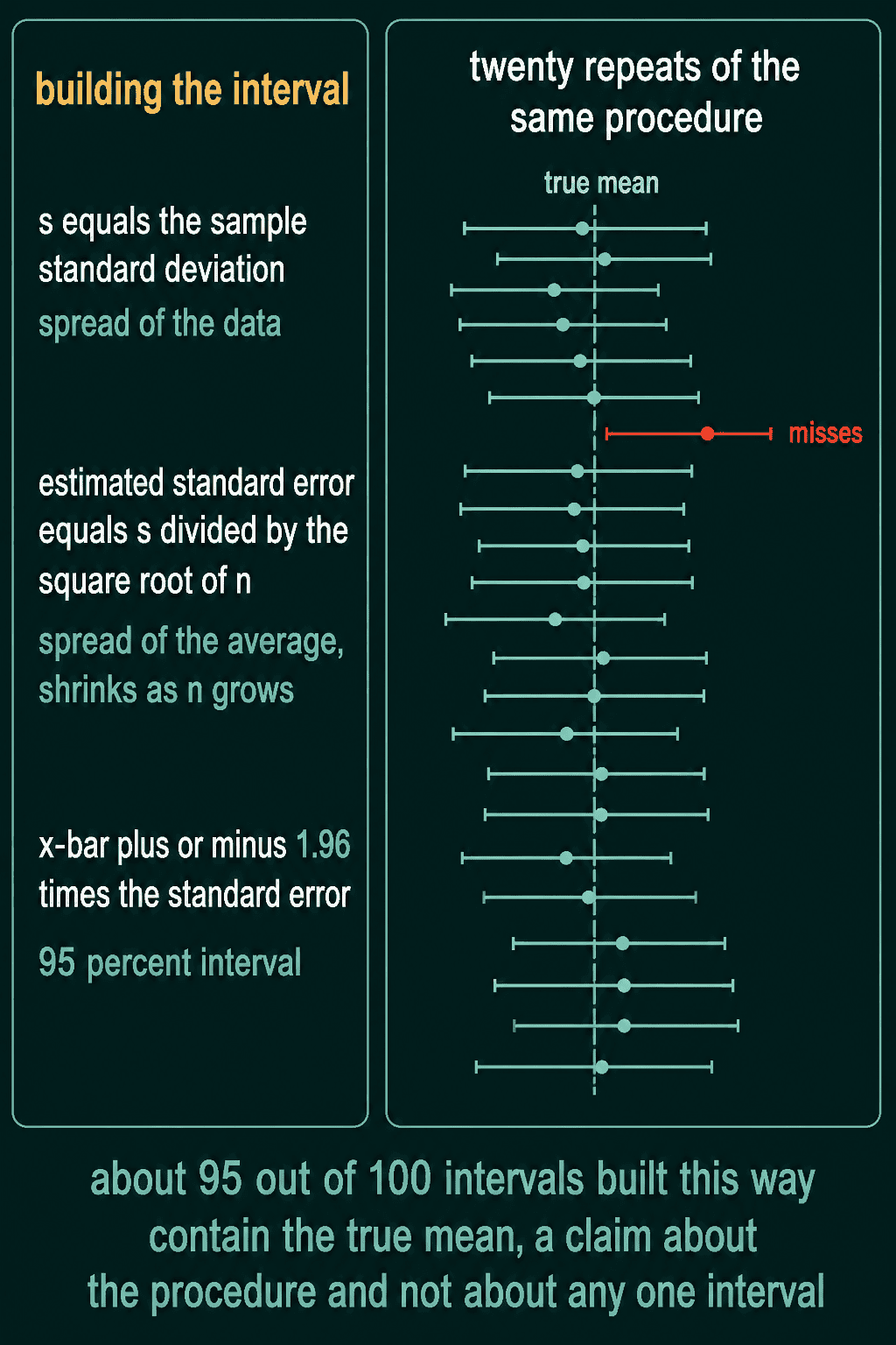
That is the same behavior the simulation above measured: 9,450 of 10,000 intervals contained the true mean.
Error bars on ML numbers
A validation accuracy is an average of 1s (correct predictions) and 0s (wrong ones), so the same formula gives it an error bar. Here is a model that gets 870 of 1,000 validation examples right:
1import torch
2
3correct = torch.cat([torch.ones(870), torch.zeros(130)])   # 870 of 1,000 right
4acc = correct.mean()
5se = correct.std() / correct.numel() ** 0.5
6print(round(acc.item(), 3), round(se.item(), 4))
7print(round((acc - 1.96 * se).item(), 3), round((acc + 1.96 * se).item(), 3))
8# 0.87 0.0106
9# 0.849 0.891
The accuracy is 0.87 with a standard error of about 0.011, so the 95% interval runs from 0.849 to 0.891. A second model scoring 0.88 on the same 1,000 examples sits inside that range, and the one-point difference between the two is well within the noise of a 1,000-example validation set.
The same goes for average latency, average loss, and the lift in an A/B test. Reporting a point estimate without its standard error makes it look more certain than it is.
When to use it, and common mistakes
Use the standard error any time you report an average computed from a sample, and reach for a confidence interval when you want to say how far off that average could be. If the numbers you are comparing come from small samples, use the t multiplier rather than 1.96.
- Dividing by $n$ instead of $\sqrt{n}$. The standard error is $s/\sqrt{n}$. Dividing by $n$ makes the error bar far too narrow.
- Using 1.96 with a handful of values. With 5 values the 1.96 interval covered the true mean only 88.5% of the time in the simulation above.
- Reading the interval as a probability statement about one interval. The 95% belongs to the procedure that built the interval, not to the one interval you got.
- Treating dependent rows as independent. Many rows from the same user carry less information than their count suggests, and so do near-duplicate examples. The estimate $s/\sqrt{n}$ then comes out too small.
Related concepts
The law of large numbers and the central limit theorem explain why averages settle down and why their error is bell-shaped with spread $\sigma/\sqrt{n}$. Degrees of freedom covers the $n-1$ divisor in more depth. The Gaussian distribution post covers the bell curve that 1.96 comes from, and CDF, percentiles and quantiles explains what a 0.975 quantile is. Hypothesis testing and p-values uses the same standard error to decide whether one model really beats another.
QuiddityML teaches standard error and confidence intervals as one concept in the Math track's probability unit, and the exercises on it include filling in a standard_error function and writing ci_95 from scratch.