By Sagi Shaier · 19 October 2026 · 6 min read

Bias and variance of an estimator, and why sample variance divides by n minus 1

How to measure an estimator's bias and variance with a simulation, how they add up to mean squared error, and how to choose between the two sample variance formulas in PyTorch.

An estimator is a rule that turns a dataset into a guess for an unknown quantity, such as the average of the data as a guess for the true mean. Its bias says whether the guess is off-center on average, and its variance says how much the guess changes from one dataset to the next. These two numbers explain why the sample variance divides by $n - 1$, and why an estimator that is slightly off-center can still be the more accurate one.

What an estimator is

Draw 5 numbers from a source whose true mean is 10 and average them. The result might be 9.4. Draw 5 new numbers and the average might be 10.7. The rule stays the same while the answer changes with the data, so an estimate is itself a random number with its own distribution.

The unknown true value is written $\theta$ (theta), and the estimate computed from the data is written $\hat{\theta}$ (theta hat). $\mathbb{E}[\hat{\theta}]$ is the expected value of the estimate: its average over many datasets of the same size. Both bias and variance are statements about that whole distribution of estimates, not about one dataset.

Bias of an estimator

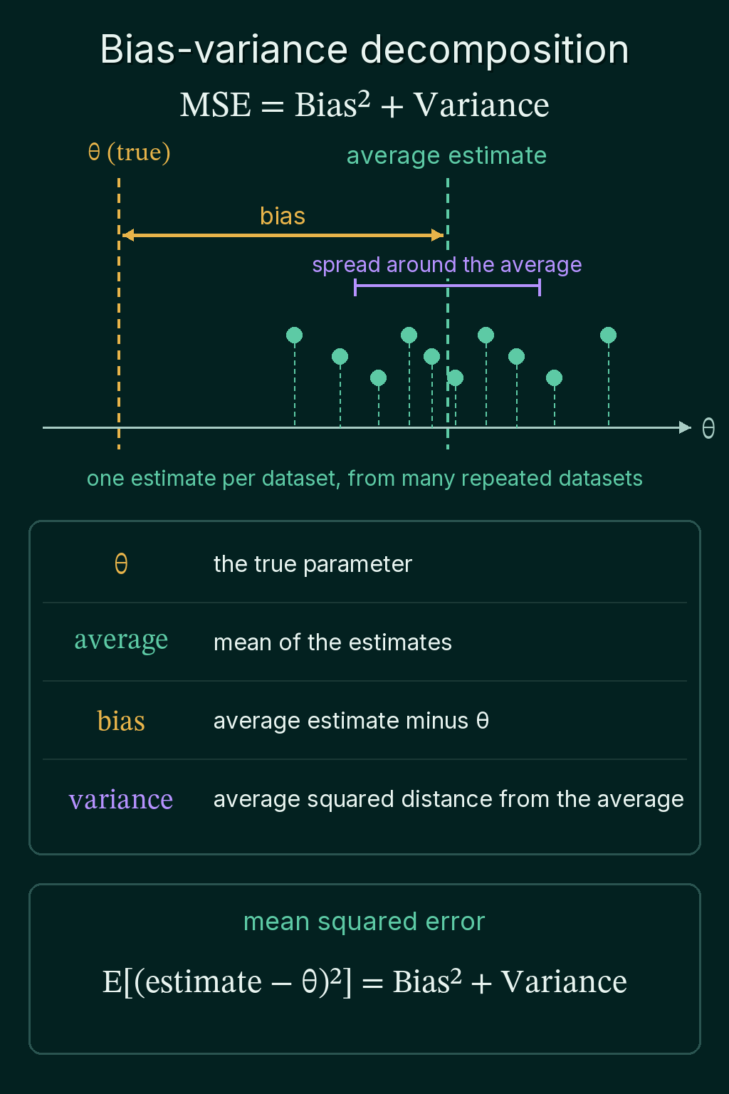
The bias of an estimator is the gap between its average and the true value:

$$\mathrm{Bias}(\hat{\theta})=\mathbb{E}[\hat{\theta}]-\theta$$

An estimator whose bias is 0 is unbiased: it can miss on any one dataset, but the misses cancel out on average. To check the sample mean, generate 200,000 datasets of 5 points each from a source with mean 10 and variance 4, and compute the sample mean of each one:

1import torch
2 
3torch.manual_seed(0)
4true_mean, true_var, n = 10.0, 4.0, 5
5data = true_mean + true_var**0.5 * torch.randn(200_000, n)   # 200,000 datasets of 5 points
6 
7means = data.mean(dim=1)                  # one sample mean per dataset
8print(round(means.mean().item(), 3))      # average of the estimates
9print(round(means.var().item(), 3))       # how much they move between datasets
10# 9.997
11# 0.799

The estimates average out to 9.997, so the sample mean is unbiased, up to simulation noise.

Variance of an estimator

The variance of an estimator measures how far the estimates spread around their own average:

$$\mathrm{Var}(\hat{\theta})=\mathbb{E}\left[(\hat{\theta}-\mathbb{E}[\hat{\theta}])^2\right]$$

For the sample means above it came out at 0.799. A mean of 5 points from a source with variance 4 has variance $4/5 = 0.8$, and more data shrinks it, which is what a standard error measures.

This is related to the bias-variance tradeoff of a model, but the question here is narrower. It is about one estimated number, like a mean or a variance: is it centered on the truth, and how much does it move from sample to sample?

Mean squared error

The overall accuracy of an estimator is its mean squared error (MSE), the average squared distance from the truth:

$$\mathrm{MSE}(\hat{\theta})=\mathbb{E}\left[(\hat{\theta}-\theta)^2\right]$$

Add and subtract $\mathbb{E}[\hat{\theta}]$ inside the square. The error $\hat{\theta} - \theta$ becomes the estimate's distance from its own average, $\hat{\theta} - \mathbb{E}[\hat{\theta}]$, plus the bias $\mathbb{E}[\hat{\theta}] - \theta$. Squaring gives the square of each part plus twice their product. The product averages to 0, because the first part averages to 0 and the bias is a fixed number. What remains is

$$\mathrm{MSE}(\hat{\theta}) = \mathrm{Bias}(\hat{\theta})^2 + \mathrm{Var}(\hat{\theta})$$

An estimator can have a small bias and still a lower total error, if its variance is smaller by more than the squared bias:

The bias-variance decomposition MSE = Bias squared + Variance, with the true theta, the average of ten estimates from repeated datasets, the bias as the distance between them, the spread of the estimates around their average, and a legend for each term.

Why sample variance divides by n minus 1

The usual way to estimate a variance is the average squared distance of the data points from their mean. The maximum likelihood estimate for a Gaussian, $\hat\sigma^2_{MLE}$, does exactly that and divides by $n$:

$$\hat\sigma^2_{MLE} = \frac{1}{n}\sum_{i=1}^n (x_i-\hat\mu)^2$$

Here $\hat\mu$ is the sample mean, and because it is computed from the same data points, the estimate comes out biased. The sample mean is the point that makes the sum of squared distances to the data as small as it can be, so the data looks a little closer to it than to the true mean. Take the values 1, 3 and 8, and suppose the true mean is 5:

1import torch
2 
3x = torch.tensor([1.0, 3.0, 8.0])
4sample_mean = x.mean()
5print(sample_mean.item())
6print(((x - sample_mean) ** 2).sum().item())   # around the sample mean
7print(((x - 5.0) ** 2).sum().item())           # around the true mean of 5
8# 4.0
9# 26.0
10# 29.0

Around the sample mean 4 the squared distances add up to 26, and around the true mean 5 they add up to 29. On average, the MLE comes out too small by a factor of $(n-1)/n$:

$$\mathbb{E}[\hat\sigma^2_{MLE}] = \frac{n-1}{n}\sigma^2$$

Dividing by $n - 1$ instead of $n$ cancels that factor, which gives an unbiased estimate:

$$\hat\sigma^2 = \frac{1}{n-1}\sum_{i=1}^n (x_i - \hat\mu)^2$$

The same kind of simulation tests both versions, with 200,000 datasets of 5 points and a true variance of 4. In PyTorch, x.var(correction=0) divides by $n$ and x.var() divides by $n - 1$:

1import torch
2 
3torch.manual_seed(0)
4true_var, n = 4.0, 5
5data = 2.0 * torch.randn(200_000, n)      # 200,000 datasets of 5 points, true variance 4
6 
7for name, correction in (("divide by n", 0), ("divide by n - 1", 1)):
8    est = data.var(dim=1, correction=correction)   # one estimate per dataset
9    mse = ((est - true_var) ** 2).mean()
10    print(f"{name:16s} average {est.mean():.2f}  variance {est.var():.2f}  mse {mse:.2f}")
11# divide by n      average 3.20  variance 5.12  mse 5.76
12# divide by n - 1  average 4.00  variance 8.00  mse 8.00

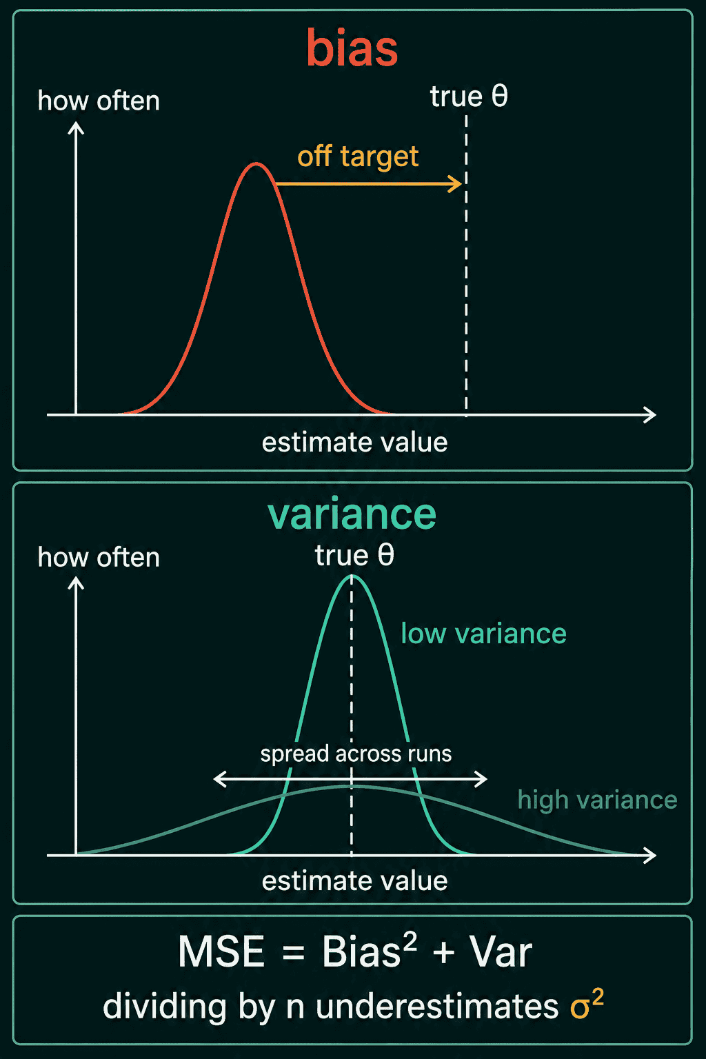
Dividing by $n$ averages 3.20, which is $4/5 \times 4$ and a bias of $-0.8$. Dividing by $n - 1$ averages 4.00, so its bias is 0. The unbiased version also moves more between datasets, with a variance of 8.00 against 5.12. Check the decomposition on the first row: $(-0.8)^2 + 5.12 = 0.64 + 5.12 = 5.76$. Here the biased estimator has the lower mean squared error, 5.76 against 8.00.

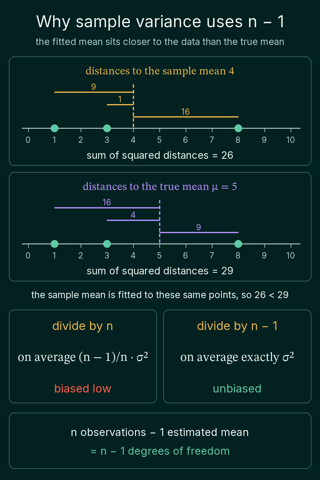
The values 1, 3 and 8 with squared distances to their sample mean 4 adding up to 26 and to a true mean of 5 adding up to 29, a box saying dividing by n is biased low, a box saying dividing by n minus 1 is unbiased, and n observations minus 1 estimated mean as n minus 1 degrees of freedom.

The two estimators answer different questions. The $n - 1$ version is the one a standard error and a confidence interval use, because they want an unbiased estimate of spread. The $n$ version is the variance that makes the observed data most probable under a Gaussian. The picture puts the three ideas side by side:

Two panels: an estimate distribution centered away from the true theta, labeled bias, and a narrow and a wide distribution centered on the true theta, labeled low and high variance, above the formula MSE = Bias squared + Var and the note that dividing by n underestimates sigma squared.

Which one to use, and common mistakes

Use the $n - 1$ version when the variance feeds a standard error, a confidence interval or a statistical test. The $n$ version is the one to use when fitting a Gaussian by maximum likelihood. With a lot of data the choice barely changes anything: at $n = 1000$ the two differ by a factor of 0.999.

Assuming unbiased means more accurate. With 5 points the unbiased variance had a mean squared error of 8.00, against 5.76 for the biased one.
Judging bias from one dataset. Bias is an average over many datasets, and one estimate that lands far from the truth says little about it.
Mixing up the PyTorch defaults. x.var() and x.std() divide by $n - 1$ unless told otherwise, and correction=0 switches them to $n$.
Confusing estimator bias with model bias. A model's bias in the bias-variance tradeoff is about how well it fits, while estimator bias is about one estimated number.

The $n - 1$ is the number of degrees of freedom left after estimating the mean. Standard error and confidence intervals are where the unbiased variance gets used. MLE vs MAP estimation derives the divide-by-$n$ formula as the Gaussian maximum likelihood estimate. The bias-variance tradeoff applies the same split to a model's prediction error.

QuiddityML teaches the bias and variance of an estimator as a concept in the Math track's probability unit, and the exercises on it include picking the code that computes the unbiased sample variance from its formula.