By Sagi Shaier · 17 October 2026 · 8 min read

The multivariate Gaussian, covariance matrices, and Mahalanobis distance

How to read and estimate a covariance matrix and how much a full or diagonal one costs to learn, plus how Mahalanobis distance flags outliers, with PyTorch code for each step.

The multivariate Gaussian is the bell-shaped distribution for a vector of numbers instead of a single number. It describes several quantities at once, like the height and weight of a person or the two coordinates of a measurement error, including how strongly they move together. It sits underneath Gaussian mixture models, Kalman filters and any model that assumes Gaussian noise on a vector. Its distance measure, the Mahalanobis distance, is a common way to flag outliers in data with more than one column.

From one dimension to many

A one-dimensional Gaussian has two parameters: a mean $\mu$ (mu) for the center and a variance $\sigma^2$ (sigma squared) for the spread. A random vector $\mathbf{X}$ with $d$ entries needs the same two things, one level up.

The mean becomes a mean vector, one mean per entry:

$$\boldsymbol{\mu} = \mathbb{E}[\mathbf{X}]$$

$\mathbb{E}[\cdot]$ means "the average value of". The variance becomes a $d \times d$ covariance matrix $\Sigma$ (capital sigma), whose entry in row $i$ and column $j$ is the covariance of entries $i$ and $j$:

$$\Sigma_{ij} = \mathrm{Cov}(X_i, X_j)$$

The covariance of two quantities is positive when they tend to be above their means together, negative when one tends to be high while the other is low, and 0 when there is no linear co-movement. The covariance of a quantity with itself is its variance. So the diagonal entries of $\Sigma$ are the variances of the individual entries, and the off-diagonal entries are the covariances between pairs.

Reading a covariance matrix

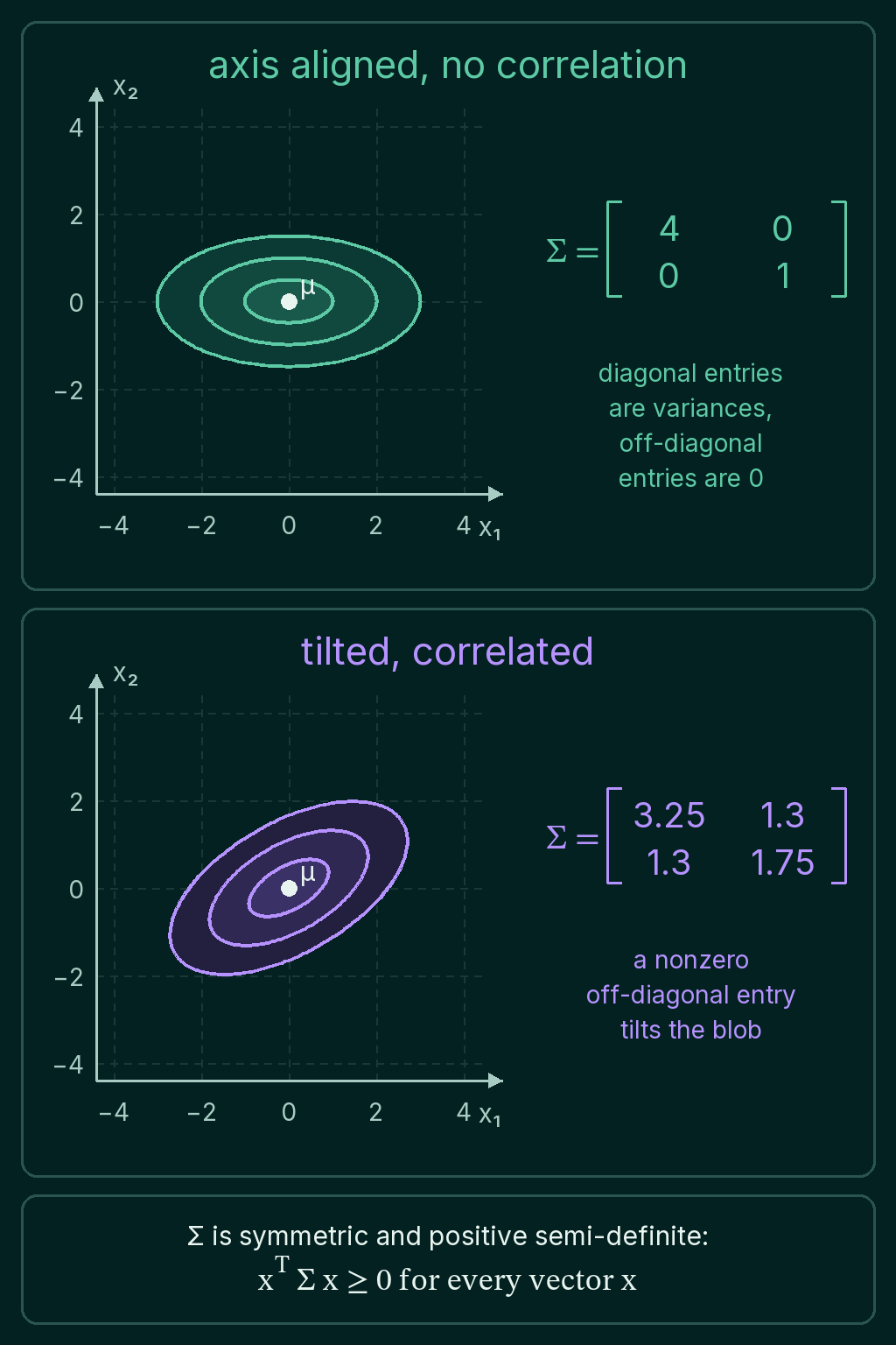
Take two examples in two dimensions, both centered at $\boldsymbol{\mu} = (0, 0)$:

$$\Sigma_A = \begin{bmatrix} 4 & 0 \\ 0 & 1 \end{bmatrix} \qquad \Sigma_B = \begin{bmatrix} 3.25 & 1.3 \\ 1.3 & 1.75 \end{bmatrix}$$

In $\Sigma_A$, the first coordinate $x_1$ has variance 4 (a standard deviation of 2) and the second coordinate $x_2$ has variance 1. The off-diagonal entries are 0, so the two coordinates do not move together. The cloud of points is stretched along $x_1$ and lines up with the axes.

In $\Sigma_B$, the off-diagonal entry 1.3 is positive, so $x_1$ and $x_2$ tend to be high together. The cloud tilts up to the right. Every covariance matrix is symmetric, $\Sigma_{ij} = \Sigma_{ji}$, because the covariance of $x_1$ with $x_2$ is the same number as the covariance of $x_2$ with $x_1$.

Two density plots with nested elliptical contours: an axis-aligned ellipse stretched along x1 for the covariance matrix with 4 and 1 on the diagonal and zeros off it, and a tilted ellipse for the matrix with 3.25, 1.3, 1.3 and 1.75, plus the note that Sigma is symmetric and positive semi-definite, which is covered later in this post.

The density

With the mean vector and the covariance matrix in hand, the density of the multivariate Gaussian at a point $\mathbf{x}$ is:

$$p(\mathbf{x}) = (2\pi)^{-d/2}\,|\Sigma|^{-1/2}$$

$$\times\exp\!\left(-\tfrac{1}{2}(\mathbf{x}-\boldsymbol{\mu})^\top\Sigma^{-1}(\mathbf{x}-\boldsymbol{\mu})\right)$$

Each piece has one job:

$\mathbf{x} - \boldsymbol{\mu}$ is how far the point is from the center, as a vector.
$\Sigma^{-1}$ is the inverse of the covariance matrix. Sandwiching it between $(\mathbf{x}-\boldsymbol{\mu})^\top$ and $(\mathbf{x}-\boldsymbol{\mu})$ turns the distance vector into one number, which is large when the point is far from the center in a direction where the data has little spread.
$|\Sigma|$ is the determinant of $\Sigma$, and together with $(2\pi)^{-d/2}$ it keeps the total probability at 1.

For $d = 1$ the formula becomes the familiar one-dimensional Gaussian: $|\Sigma|$ is $\sigma^2$ and $\Sigma^{-1}$ is $1/\sigma^2$, so the exponent is $-(x-\mu)^2/(2\sigma^2)$.

Points with the same value of the number in the exponent have the same density, and those points form an ellipse. That is why the contour lines in the picture are ellipses. For $\Sigma_B$ the ellipses tilt at 30 degrees, and they are twice as long as they are wide, because the eigenvalues of $\Sigma_B$ are 4 and 1.

Estimating the mean and covariance from data

For a data matrix X with one row per sample and one column per dimension, X.mean(dim=0) gives $\boldsymbol{\mu}$, and centered = X - X.mean(dim=0) subtracts it from every row. Then centered.T @ centered / X.shape[0] gives $\Sigma$, where @ is matrix multiplication and X.shape[0] is the number of samples. Draw 50,000 points from a Gaussian with covariance $\Sigma_B$ and the estimate lands close to it:

1import torch
2 
3torch.manual_seed(0)
4true_cov = torch.tensor([[3.25, 1.3], [1.3, 1.75]])
5X = torch.distributions.MultivariateNormal(torch.zeros(2), true_cov).sample((50_000,))
6 
7mu = X.mean(dim=0)
8centered = X - mu
9sigma = centered.T @ centered / X.shape[0]
10print(mu)
11print(sigma)
12# tensor([-0.0051, -0.0043])
13# tensor([[3.2485, 1.3104],
14#         [1.3104, 1.7652]])

Entry $(i, j)$ of centered.T @ centered is the sum over samples of the product of the centered values in columns $i$ and $j$. Dividing by the number of samples turns that sum into the average product, which is the covariance.

The log of the density is what code usually evaluates. torch.linalg.inv(sigma) computes $\Sigma^{-1}$ and torch.logdet(sigma) computes $\log|\Sigma|$. Written out by hand, the log-density matches PyTorch's MultivariateNormal:

1import math
2import torch
3from torch.distributions import MultivariateNormal
4 
5mu = torch.tensor([0.0, 0.0])
6sigma = torch.tensor([[3.25, 1.3], [1.3, 1.75]])
7 
8def gaussian_log_density(x, mu, sigma):
9    d = x.shape[0]
10    diff = x - mu
11    quad = diff @ torch.linalg.inv(sigma) @ diff
12    return -0.5 * (d * math.log(2 * math.pi) + torch.logdet(sigma) + quad)
13 
14x = torch.tensor([2.0, 2.0])
15print(gaussian_log_density(x, mu, sigma))
16print(MultivariateNormal(mu, sigma).log_prob(x))
17print(torch.det(sigma), torch.linalg.eigvalsh(sigma))
18# tensor(-3.7315)
19# tensor(-3.7315)
20# tensor(3.9975) tensor([0.9992, 4.0008])

The last line confirms the shape: the determinant is about 4 and the eigenvalues are about 1 and 4.

Positive semi-definite and positive definite

A covariance matrix is positive semi-definite (PSD), which means

$$\mathbf{v}^\top \Sigma\,\mathbf{v} \ge 0 \quad \text{for every vector } \mathbf{v}$$

For a vector $\mathbf{v}$ of length 1, the number $\mathbf{v}^\top \Sigma\,\mathbf{v}$ is the variance of the data along $\mathbf{v}$, so the condition says no direction can have negative variance. When no direction has exactly zero variance, $\Sigma$ is positive definite. That stronger condition also makes $\Sigma$ invertible, so the density formula can use $\Sigma^{-1}$.

A covariance matrix that is not invertible, called singular, means some direction in the data has no spread at all. It happens when one feature is an exact multiple of another, like the same length stored once in meters and once in centimeters. Then $\Sigma^{-1}$ does not exist and the density formula breaks.

Covariance budgets

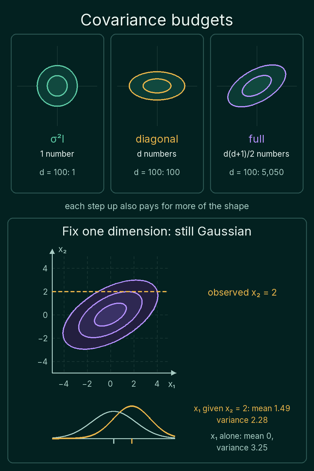
A full covariance matrix has $d^2$ entries, but because it is symmetric only $d(d+1)/2$ of them are independent: the diagonal plus one triangle. That count grows fast. For $d = 100$ it is 5,050 numbers, and each one has to be estimated from data. So models choose how much of the matrix to learn:

Isotropic covariance, $\Sigma = \sigma^2 I$, where $I$ is the identity matrix: 1 number. Every direction gets the same spread and nothing is correlated, so the contours are circles.
Diagonal covariance: $d$ numbers, one variance per dimension, with every off-diagonal entry fixed at 0. The contours are ellipses lined up with the axes.
Full covariance: $d(d+1)/2$ numbers, which also pay for the correlations. The contours can tilt.

Models that fit Gaussians to high-dimensional data often settle for the diagonal option, because estimating the full matrix reliably needs much more data. Other middle grounds shrink a full matrix toward a diagonal one, or model it as a low-rank matrix plus a diagonal.

What stays Gaussian

Two results make the multivariate Gaussian convenient to compute with.

First, fix some dimensions to known values and the remaining dimensions are still Gaussian, with a mean and covariance that shift toward the observed values. For $\Sigma_B$, observing $x_2 = 2$ leaves $x_1$ Gaussian with mean 1.49 and variance 2.28. Before the observation, $x_1$ had mean 0 and variance 3.25. A simulation that keeps only the points with $x_2$ close to 2 agrees:

1import torch
2 
3torch.manual_seed(0)
4sigma = torch.tensor([[3.25, 1.3], [1.3, 1.75]])
5X = torch.distributions.MultivariateNormal(torch.zeros(2), sigma).sample((5_000_000,))
6 
7slice_ = X[(X[:, 1] - 2.0).abs() < 0.02]     # keep points with x2 close to 2
8print(len(slice_), slice_[:, 0].mean(), slice_[:, 0].var())
9# 19229 tensor(1.4951) tensor(2.2964)

The mean moved up because $x_1$ and $x_2$ have positive covariance, so a high $x_2$ suggests a high $x_1$. The variance dropped because knowing $x_2$ removes some of the uncertainty about $x_1$.

Second, if $\mathbf{x}$ is Gaussian and $\mathbf{y}$ is a linear function of $\mathbf{x}$ plus Gaussian noise, then $\mathbf{x}$ given $\mathbf{y}$ is also Gaussian in closed form. Kalman filters and Gaussian processes rely on these two facts: everything stays Gaussian at every step, so the computation reduces to matrix algebra.

Three panels with one ring each for an isotropic covariance costing 1 number, a diagonal covariance costing d numbers and a full covariance costing d(d+1)/2 numbers, or 5,050 at d = 100, and below a tilted Gaussian sliced at x2 = 2 with the slice's distribution of x1 shifted to mean 1.49 and variance 2.28.

Mahalanobis distance

The number inside the exponent of the density is also a distance. The Mahalanobis distance of a point $\mathbf{x}$ from the mean is its square root:

$$D_M(\mathbf{x}) = \sqrt{(\mathbf{x}-\boldsymbol{\mu})^\top \Sigma^{-1} (\mathbf{x}-\boldsymbol{\mu})}$$

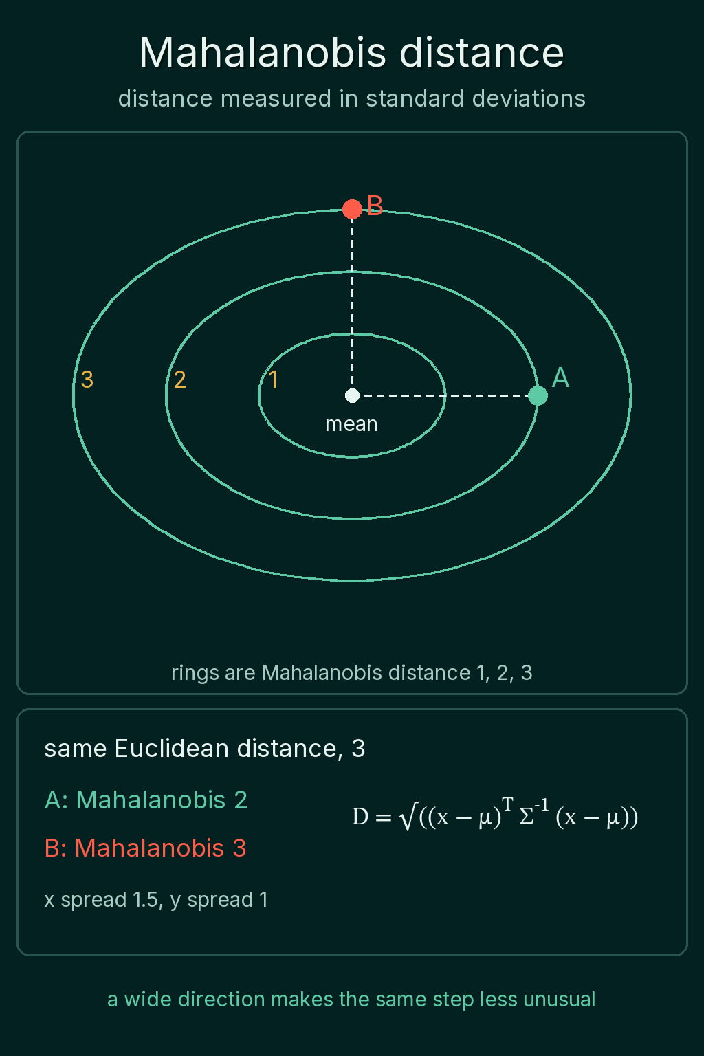
Ordinary Euclidean distance, $\|\mathbf{x}-\boldsymbol{\mu}\|$, is the straight-line length and treats every direction the same. Mahalanobis distance divides out $\Sigma$, so it counts distance in standard deviations along each direction. A step along a direction where the data is tightly packed counts as more unusual than the same step along a direction where the data is spread out. Because the density depends on $\mathbf{x}$ only through this number, points at the same Mahalanobis distance have the same density, and the density contours are rings of constant Mahalanobis distance.

Take $\Sigma = \begin{bmatrix} 2.25 & 0 \\ 0 & 1 \end{bmatrix}$, a standard deviation of 1.5 along $x_1$ and 1 along $x_2$. Point $A = (3, 0)$ and point $B = (0, 3)$ are both 3 away from the mean in Euclidean distance. Along $x_1$, a distance of 3 is $3 / 1.5 = 2$ standard deviations, and along $x_2$ it is $3 / 1 = 3$. So $A$ has Mahalanobis distance 2 and $B$ has 3, and $B$ is the more unusual point:

Rings of Mahalanobis distance 1, 2 and 3 around the mean of a distribution that is wider along x1, with point A at distance 3 along x1 sitting on ring 2 and point B at distance 3 along x2 sitting on ring 3.

1import torch
2 
3def mahalanobis(x, mu, sigma):
4    diff = x - mu
5    return torch.sqrt(diff @ torch.linalg.inv(sigma) @ diff)
6 
7mu = torch.tensor([0.0, 0.0])
8sigma = torch.tensor([[2.25, 0.0], [0.0, 1.0]])
9a = torch.tensor([3.0, 0.0])
10b = torch.tensor([0.0, 3.0])
11print(torch.linalg.norm(a - mu), torch.linalg.norm(b - mu))
12print(mahalanobis(a, mu, sigma), mahalanobis(b, mu, sigma))
13 
14tilted = torch.tensor([[3.25, 1.3], [1.3, 1.75]])
15c = torch.tensor([2.0, 2.0])
16e = torch.tensor([2.0, -2.0])
17print(mahalanobis(c, mu, tilted), mahalanobis(e, mu, tilted))
18# tensor(3.) tensor(3.)
19# tensor(2.) tensor(3.)
20# tensor(1.5497) tensor(2.7577)

The last line uses the tilted $\Sigma_B$. The points $(2, 2)$ and $(2, -2)$ are the same Euclidean distance from the center. $(2, 2)$ lies along the tilt, where the data is spread out, and has Mahalanobis distance 1.55. $(2, -2)$ goes against the tilt and has 2.76. For flagging outliers in data with several columns, this is the property that makes Mahalanobis distance more useful than Euclidean distance: a point that breaks the usual relationship between the columns stands out even when no single column is extreme.

Common mistakes

Using a singular covariance matrix. A feature that is an exact copy or multiple of another makes $\Sigma$ non-invertible, and torch.linalg.inv fails or returns huge numbers. Remove the duplicate feature first.
Fitting a full covariance with too little data. With $d = 100$, a full matrix has 5,050 numbers to estimate. A diagonal covariance is the safer default when samples are scarce.
Computing the density instead of the log-density. In many dimensions the density can be so small that it underflows to 0. Work with log_prob and torch.logdet.
Using Euclidean distance for outliers on correlated data. It ignores both the different spreads and the tilt, so it misses points that break the correlation.

The Gaussian distribution post covers the one-dimensional case, including why code uses the log-density. Covariance vs correlation explains the entries that fill the covariance matrix. Eigenvalues and eigenvectors give the axes and lengths of the density's ellipses, and positive definite matrices covers the condition that makes $\Sigma$ invertible.

QuiddityML teaches the multivariate Gaussian and Mahalanobis distance as two concepts in the Math track's probability unit, and the exercises on them include picking the code block that computes the log-density, writing covariance_matrix from scratch and choosing why Mahalanobis distance flags outliers better than Euclidean distance.