By Sagi Shaier · 18 October 2026 · 8 min read
Hypothesis testing and p-values: is model A really better than model B?
How to tell whether a gap between two models is real or noise, what a p-value does and does not mean, one-sided vs two-sided tests, and why running many tests produces false winners, with PyTorch checks.
A hypothesis test checks whether your data is surprising under a baseline claim, called the null hypothesis. The p-value is the number the test produces: the probability of seeing a result at least as extreme as yours if the null hypothesis were true. In ML the question is usually whether a new model beats an old one, and a test answers it by comparing the gap between their scores with the amount of noise in those scores.
The null hypothesis
The null hypothesis is the boring explanation, written as a specific claim. If a new model scores 82% and the old one 80%, the null hypothesis is that the two models have the same true accuracy and the 2-point gap came from which examples happened to be in the test set. The test asks how unusual a 2-point gap would be if that were the case.
The null is written $H_0$. The claim you would conclude if the data rules out the null is called the alternative hypothesis, $H_1$. Here $H_1$ says the new model's true accuracy is different from the old one's.
Measuring a gap in standard errors
A 2-point gap can be large or tiny depending on how noisy the scores are. Any score computed from a test set has a standard error: how much it would move if you evaluated on a fresh test set of the same size. The test divides the gap by that standard error:
$$z = \frac{\hat{\theta} - \theta_0}{\widehat{\mathrm{SE}}}$$
$\hat{\theta}$ (theta hat) is the estimate from your data, here the observed accuracy gap of 0.02. $\theta_0$ is the value the null hypothesis claims, here a gap of 0. $\widehat{\mathrm{SE}}$ is the estimated standard error of the gap. The result $z$ is called the test statistic: the gap measured in standard errors.
Suppose the standard error of the gap is 0.005, half a percentage point. Then
$$z = \frac{0.02 - 0}{0.005} = 4$$
The gap is 4 standard errors from zero. If the same 0.02 gap came with a standard error of 0.02, $z$ would be 1, and a gap of one standard error happens by chance often. The denominator decides how big a gap has to be to count.
The p-value
If the null hypothesis is true, $z$ follows the standard Gaussian, the bell curve with mean 0 and standard deviation 1. The p-value is the area under that curve at least as far out as the observed $z$:
$$p = P(\text{data at least this extreme} \mid H_0 \text{ is true})$$
The vertical bar reads "given". The picture shows an observed $z$ of 2.6. The shaded tail beyond it holds about 0.5% of the area:
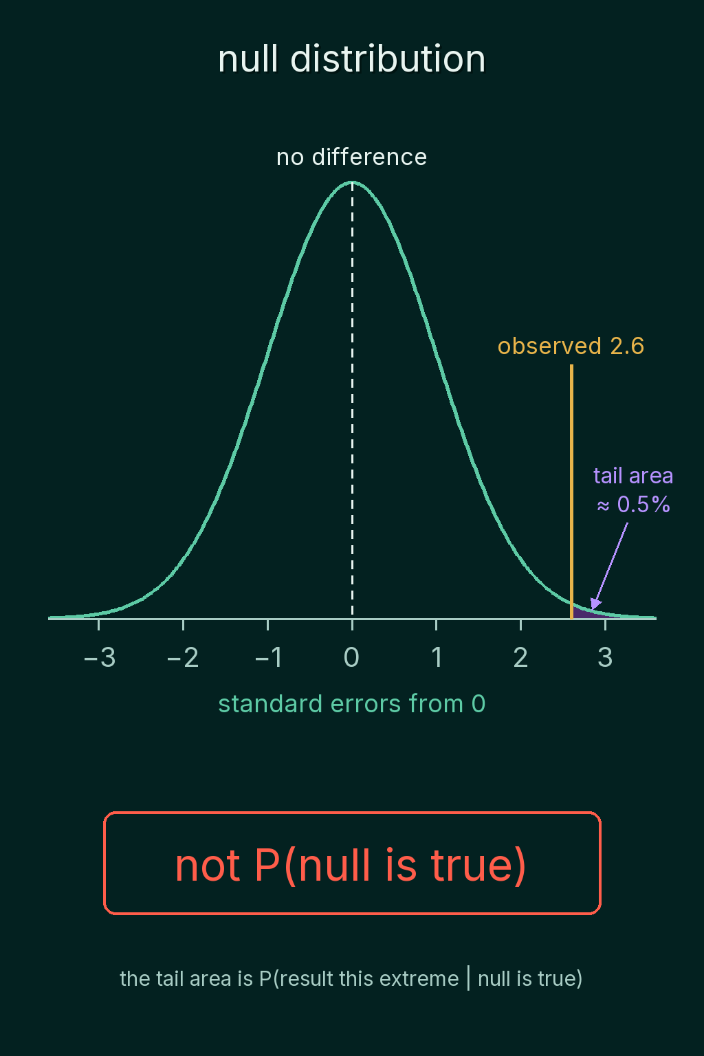
Normal(0, 1).cdf(z) gives the area to the left of $z$, so one minus it is the area to the right. For the 82% vs 80% example, with a gap of 4 standard errors, both tails together give the p-value:
1import torch
2from torch.distributions import Normal
3
4std_normal = Normal(0.0, 1.0)
5
6new_acc, old_acc, se_gap = 0.82, 0.80, 0.005
7z = (new_acc - old_acc) / se_gap
8p_two_sided = 2 * (1 - std_normal.cdf(torch.tensor(abs(z))))
9print(round(z, 2), f"{p_two_sided.item():.2g}")
10# 4.0 6.3e-05
A p-value of 0.000063 says that if the two models were equally accurate, a gap this large would show up about 6 times in 100,000 evaluations. The next section explains why this example counts both tails.
What a p-value does not mean
A p-value of 0.03 does not mean there is a 3% probability that the null hypothesis is true. It means that if the null were true, results at least this extreme would happen about 3% of the time. The two sound alike, and they are different probabilities: the p-value is computed assuming the null is true, so it cannot also be the probability that the null is true.
A small p-value also does not prove the alternative. It says the data and the null hypothesis fit together poorly, under the assumptions the test makes, such as independent test examples.
One-sided and two-sided tests
"At least this extreme" can mean two things, and you pick one before looking at the data. A two-sided test counts a gap of that size in either direction. A one-sided test counts it only in the direction you predicted, for example only "the new model is better".
For the same observed $z = 2.3$, the one-sided p-value is half the two-sided one:
1import torch
2from torch.distributions import Normal
3
4std_normal = Normal(0.0, 1.0)
5z = torch.tensor(2.3)
6one_sided = 1 - std_normal.cdf(z)
7print(round(one_sided.item(), 4), round(2 * one_sided.item(), 4))
8# 0.0107 0.0214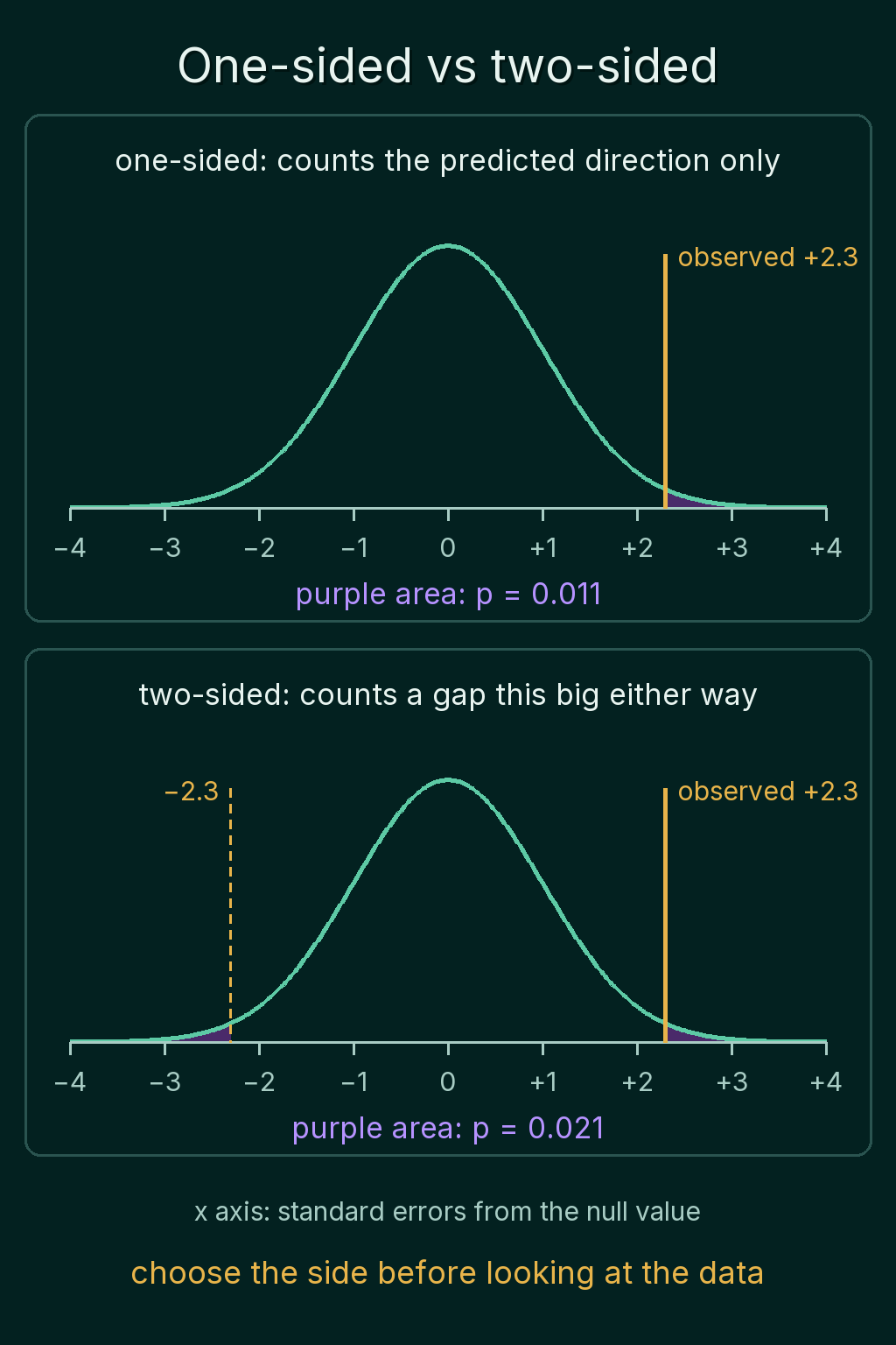
Choosing the side after seeing which way the gap went changes the test after seeing the answer, which halves the p-value for free. That is one form of p-hacking: adjusting the analysis until the p-value looks good. When in doubt, use two-sided.
Significance level and the two kinds of error
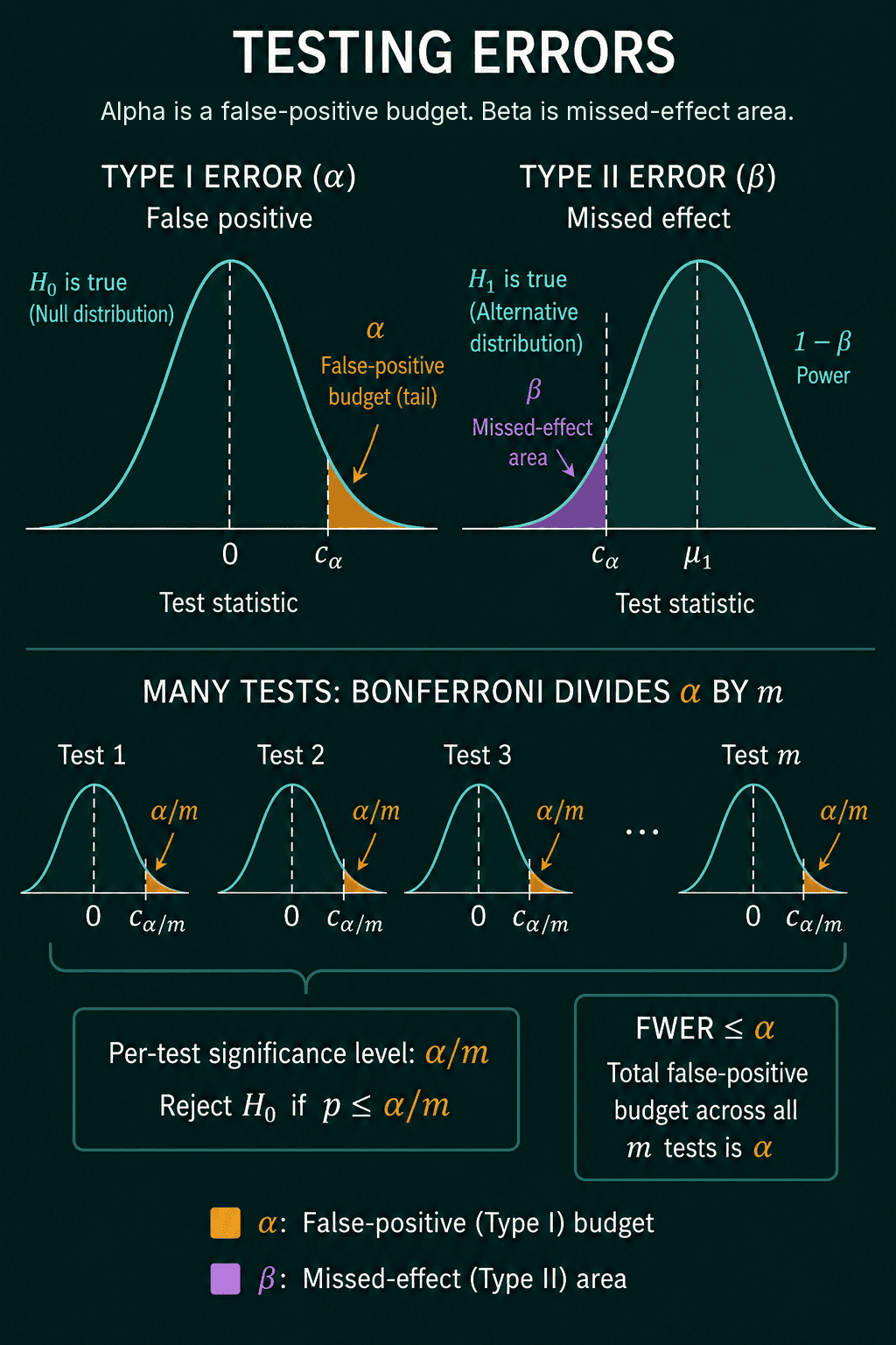
Before looking at the data, you also pick a significance level $\alpha$ (alpha), the cutoff for "surprising enough". 0.05 is a common choice. If the p-value falls below $\alpha$, you reject the null hypothesis. Otherwise you fail to reject it, which is not the same as showing it is true. A model comparison with a p-value of 0.4 has not shown the models are equal. It has only failed to show they differ.
$\alpha$ is a budget for one specific mistake. When the null hypothesis is true, the test still rejects it a fraction $\alpha$ of the time by chance. In terms of the test statistic, $\alpha$ sets a cutoff $c_\alpha$, and the null is rejected when the statistic lands beyond it. That mistake is a Type I error, or false positive: declaring a winner when there is none. The opposite mistake, missing a real difference, is a Type II error. One minus the Type II error rate is the test's power, the chance of catching a real difference when there is one.
Confidence intervals and tests give the same verdict. A 95% confidence interval for the gap that excludes zero is the same finding as $p < 0.05$ for a two-sided test against "no difference".
Many tests spend the budget many times
Each test at $\alpha = 0.05$ has a 5% chance of a false positive. Run $m$ independent tests where every null hypothesis is true, and the chance that at least one of them comes out "significant" is
$$1 - (1 - \alpha)^m$$
This chance of at least one false positive across a group of tests is called the family-wise error rate (FWER). For 20 tests it is $1 - 0.95^{20} = 0.64$. Compare 20 model variants against a baseline when none of them is really better, and nearly two times in three at least one looks like a winner. The Bonferroni correction controls this by testing each comparison at $\alpha/m$ instead, here $0.05/20 = 0.0025$. A simulation of 10,000 such experiments agrees with both numbers:
1import torch
2from torch.distributions import Normal
3
4torch.manual_seed(0)
5std_normal = Normal(0.0, 1.0)
6alpha, m, experiments = 0.05, 20, 10_000
7
8z = torch.randn(experiments, m)              # 20 tests, every null is true
9p = 2 * (1 - std_normal.cdf(z.abs()))
10
11print(round(1 - (1 - alpha) ** m, 3))
12print(round((p < alpha).any(dim=1).float().mean().item(), 3))
13print(round((p < alpha / m).any(dim=1).float().mean().item(), 3))
14# 0.642
15# 0.642
16# 0.052
Without a correction, 64.2% of the experiments produce at least one false winner. With Bonferroni, 5.2% do, back near the 5% budget.
Comparing two models
For two models evaluated on separate test sets, each accuracy has a standard error of $\sqrt{a(1-a)/n}$, where $a$ is the accuracy and $n$ the number of test examples. Independent standard errors combine as the square root of the sum of their squares. Here is the same 2.8-point gap between models scoring 0.742 and 0.714, first with 500 test examples each and then with 10,000:
1import torch
2from torch.distributions import Normal
3
4std_normal = Normal(0.0, 1.0)
5
6def compare(acc_a, acc_b, n):
7    """z and two-sided p for two accuracies, each from its own n test examples."""
8    se_a = (acc_a * (1 - acc_a) / n) ** 0.5
9    se_b = (acc_b * (1 - acc_b) / n) ** 0.5
10    se_gap = (se_a ** 2 + se_b ** 2) ** 0.5
11    z = (acc_a - acc_b) / se_gap
12    p = 2 * (1 - std_normal.cdf(torch.tensor(abs(z))))
13    return round(se_gap, 4), round(z, 2), f"{p.item():.2g}"
14
15print(*compare(0.742, 0.714, 500))
16print(*compare(0.742, 0.714, 10_000))
17# 0.0281 1.0 0.32
18# 0.0063 4.45 8.6e-06
With 500 examples the gap is one standard error and $p = 0.32$, well within the noise. With 10,000 examples the same gap is 4.45 standard errors and $p$ is about 0.0000086:
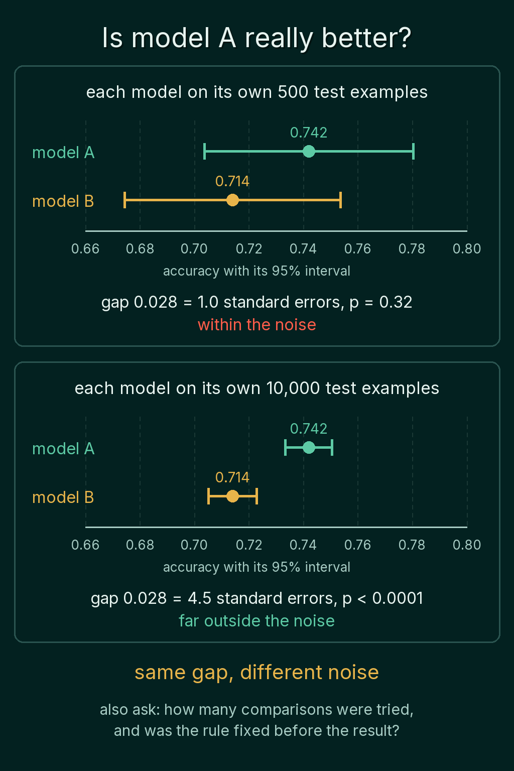
What decides it is whether the gap is large compared with the noise, not which number is bigger.
When to use it, and common mistakes
ML work uses formal p-values less than some sciences do, but the reasoning carries over to A/B tests and benchmark comparisons. It applies to any claim that one model is better than another. Before trusting a comparison, ask what was compared and how large the uncertainty was. Then ask how many comparisons were tried and whether the decision rule was fixed before the results came in.
- Reading the p-value as the probability the null is true. It is the probability of data this extreme assuming the null is true.
- Treating "not significant" as "no difference". Failing to reject the null on a small test set often means the test set was too small to tell.
- Picking the side of the test after seeing the result. That halves the p-value without any new evidence.
- Reporting the best of many comparisons. With 20 tries, a false winner shows up 64% of the time. Correct for the number of tests, or confirm the winner on fresh data.
Related concepts
Standard error and confidence intervals covers the standard error that the test statistic divides by, and the confidence interval that gives the same verdict as the test. The Gaussian distribution post explains z-scores and the bell curve the p-value is read from. The law of large numbers and the central limit theorem explain why an accuracy computed on many examples has an approximately Gaussian error in the first place.
QuiddityML teaches hypothesis tests and p-values as one concept in the Math track's probability unit, and the exercises on it include reading what p = 0.03 does and does not say and completing a z_stat function that measures the gap between two accuracies in standard errors.