By Sagi Shaier · 17 October 2026 · 7 min read

The law of large numbers and the central limit theorem explained

Why sample averages settle toward the true mean and why their error is bell-shaped with a spread of sigma over root n, plus when neither result holds, with PyTorch simulations of each.

The law of large numbers says that the average of many random samples gets close to the true average of the distribution they come from. The central limit theorem adds how close: the error of that average follows a bell curve whose width shrinks with the square root of the number of samples. Together they are why more data gives more reliable estimates, and why a validation accuracy or an average latency can be given an error bar.

Expectations have to be estimated

The expected value $\mathbb{E}[X]$ of a random quantity $X$ is its probability-weighted average, the value it comes out at on average. For a fair coin scored 1 for heads and 0 for tails, $\mathbb{E}[X] = 0.5$. In practice you rarely know the expected value of the thing you care about, like the average loss of a model on all possible inputs. You have samples, and you average them.

Write $n$ samples as $X_1, X_2, \dots, X_n$. They are independent and identically distributed (i.i.d.): each comes from the same distribution, and knowing one tells you nothing about the others. Their sample average is

$$\bar{X}_n = \frac{1}{n}\sum_{i=1}^{n} X_i$$

The bar over $X$ marks an average, and the subscript $n$ is how many samples went into it.

The law of large numbers

As $n$ grows, $\bar{X}_n$ gets closer to $\mathbb{E}[X]$. Ten coin flips can easily come out 8 heads and 2 tails, a sample average of 0.8. After 100,000 flips, the fraction of heads for a fair coin is close to 0.5:

1import torch
2 
3torch.manual_seed(0)
4flips = torch.randint(0, 2, (100_000,)).float()
5running = flips.cumsum(dim=0) / torch.arange(1, len(flips) + 1)
6 
7for n in (10, 100, 1_000, 10_000, 100_000):
8    print(n, round(running[n - 1].item(), 4))
9# 10 0.8
10# 100 0.56
11# 1000 0.504
12# 10000 0.5085
13# 100000 0.5006

flips.cumsum(dim=0) is the running count of heads, and dividing by $1, 2, \dots, n$ turns it into the running average. The picture below is a different run of the same experiment, with the number of flips on a log scale so that 10, 100 and 1,000 flips get equal room:

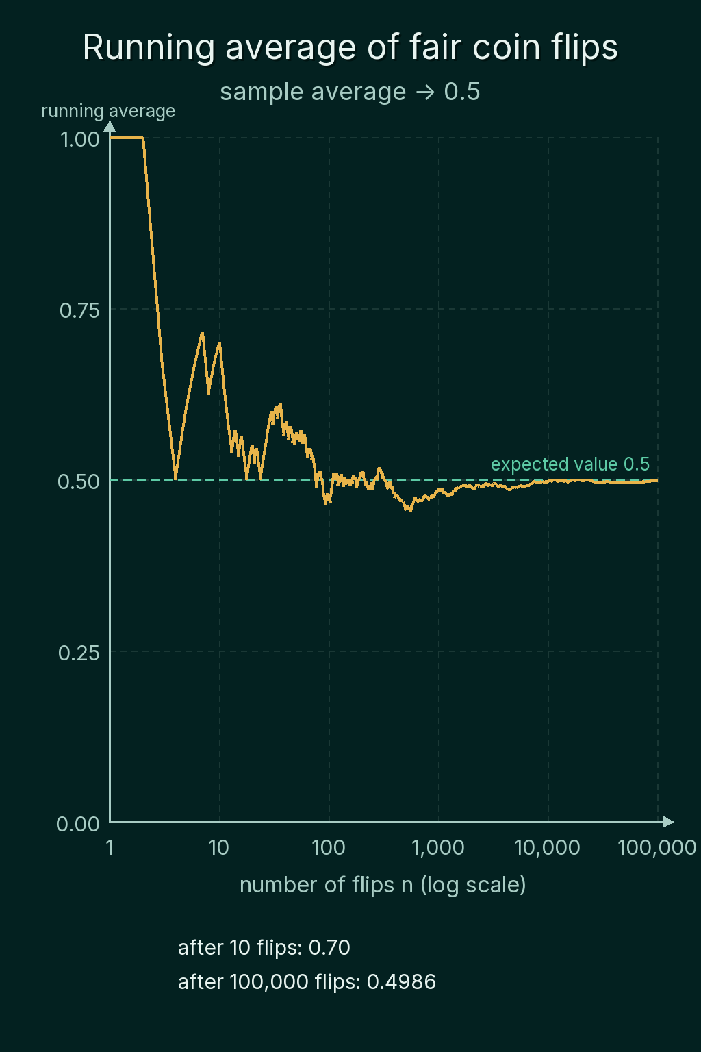
The running average of 100,000 simulated fair coin flips on a log-scale x axis, swinging between 0.5 and 1 in the first few dozen flips and settling onto the expected value 0.5, at 0.70 after 10 flips and 0.4986 after 100,000.

More precisely, pick any tolerance $\epsilon$ (epsilon), like 0.01. The probability that $\bar{X}_n$ lands further than $\epsilon$ from $\mathbb{E}[X]$ goes to 0 as $n$ grows. The law does not say the average is ever exactly right, and it says nothing about how fast it gets close. The 10,000-flip average above (0.5085) is a little further from 0.5 than the 1,000-flip one, which the law allows.

The law needs the expected value to exist. For distributions with tails so heavy that $\mathbb{E}[X]$ is undefined, sample averages never settle down. An example appears near the end of this post.

Monte Carlo estimation

The same idea gives a general way to compute expectations that are hard to work out on paper: draw many random samples and average them. This is called Monte Carlo estimation. As a check, for $U$ drawn uniformly between 0 and 1, the exact value of $\mathbb{E}[U^2]$ is $1/3 = 0.3333$:

1import torch
2 
3torch.manual_seed(0)
4u = torch.rand(1_000_000)
5for n in (100, 10_000, 1_000_000):
6    print(n, round((u[:n] ** 2).mean().item(), 4))
7# 100 0.3244
8# 10000 0.3332
9# 1000000 0.3336

The estimate from 100 samples is off in the second decimal, and the estimates from 10,000 and 1,000,000 are off in the fourth.

The central limit theorem

The law of large numbers says the average gets close. The central limit theorem (CLT) describes the error that remains. Suppose the samples are i.i.d. with mean $\mu$ (mu) and a finite variance $\sigma^2$ (sigma squared). For large $n$, the sample average is approximately Gaussian:

$$\bar{X}_n \approx \mathcal{N}\!\left(\mu, \frac{\sigma^2}{n}\right)$$

$\mathcal{N}(\mu, \sigma^2/n)$ is the bell curve centered at $\mu$ with variance $\sigma^2/n$.

The individual values do not have to be Gaussian. They can be skewed, discrete or oddly shaped, and the average still looks roughly bell-shaped, because combining many independent draws smooths out the irregular shape.

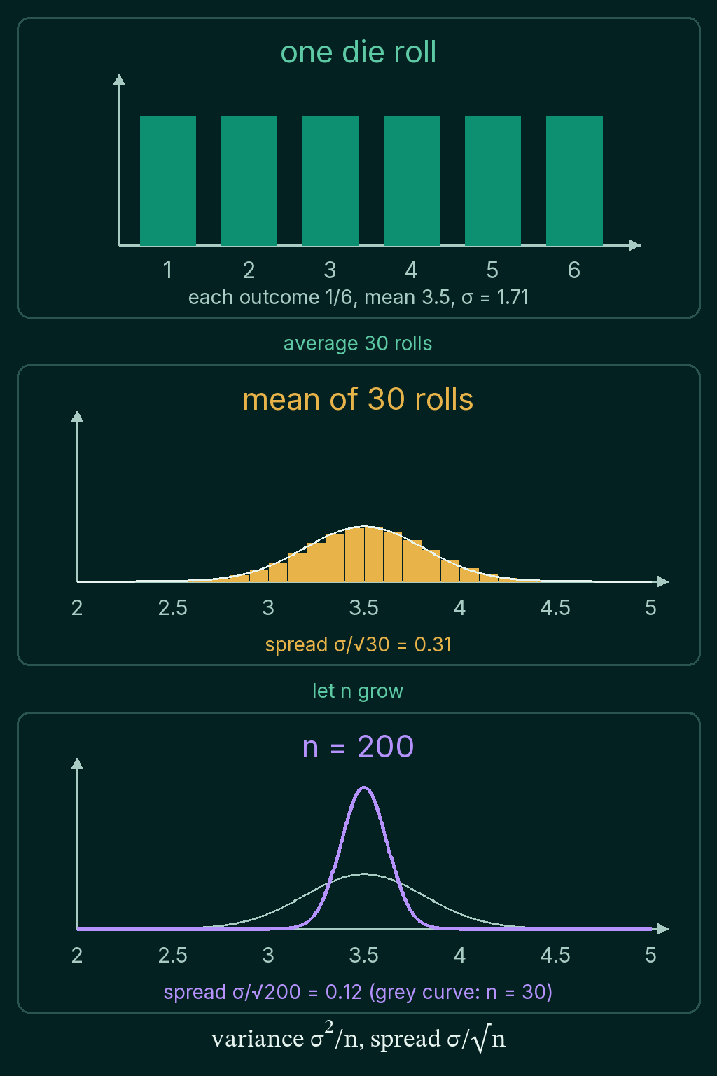
Take one roll of a fair die. The six outcomes are equally likely, a flat distribution with mean 3.5 and standard deviation $\sigma = \sqrt{35/12} = 1.708$. Average 30 rolls and repeat that 10,000 times:

1import torch
2 
3torch.manual_seed(0)
4draws = torch.randint(1, 7, (10_000, 30)).float()   # 10,000 samples of 30 rolls
5means = draws.mean(dim=1)                            # one average per sample
6 
7sigma = (35 / 12) ** 0.5
8print(round(sigma, 3), round(sigma / 30 ** 0.5, 3))
9print(round(means.mean().item(), 3), round(means.std().item(), 3))
10inside = ((means - 3.5).abs() < 1.96 * sigma / 30 ** 0.5).float().mean()
11print(round(inside.item(), 3))
12# 1.708 0.312
13# 3.503 0.315
14# 0.95

The 10,000 averages center on 3.5 with a spread of 0.315, close to the 0.312 the CLT predicts. A Gaussian puts 95% of its probability within 1.96 standard deviations of its center, and 95% of the averages land there.

One die roll with six equal bars, the exact distribution of the mean of 30 rolls as a bell-shaped histogram around 3.5 with spread 0.31, and the much narrower bell curve for the mean of 200 rolls with spread 0.12.

Why the spread is sigma over root n

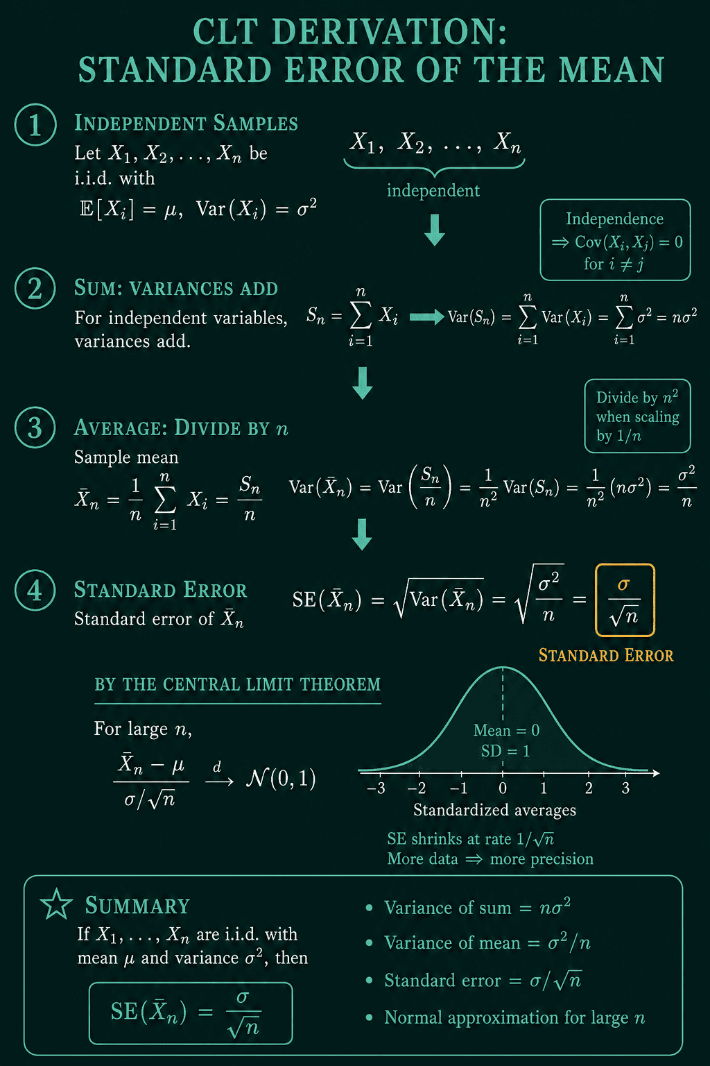
The width of that bell curve follows from how variances add. Each draw has variance $\sigma^2$. The variance of a sum of independent quantities is the sum of their variances, so the sum of $n$ draws has variance $n\sigma^2$. Dividing by $n$ to get the average divides the variance by $n^2$, because scaling a quantity by a constant scales its variance by the square of that constant. That leaves

$$\mathrm{Var}(\bar{X}_n) = \frac{\sigma^2}{n}$$

Taking the square root, the spread of the sample average is $\sigma/\sqrt{n}$. That spread is called the standard error.

The square root sets the price of precision. Four times as much data halves the standard error, and 100 times as much data cuts it to a tenth:

1import torch
2 
3torch.manual_seed(0)
4sigma = (35 / 12) ** 0.5
5for n in (30, 120, 480):
6    means = torch.randint(1, 7, (10_000, n)).float().mean(dim=1)
7    print(n, round(means.std().item(), 3), round(sigma / n ** 0.5, 3))
8# 30 0.315 0.312
9# 120 0.156 0.156
10# 480 0.078 0.078

Each step multiplies the data by 4 and halves the spread. The theorem is often written in a standardized form: subtract $\mu$ and divide by the standard error, and the result approaches the standard normal $\mathcal{N}(0, 1)$, the bell curve with mean 0 and standard deviation 1:

$$\frac{\bar{X}_n - \mu}{\sigma/\sqrt{n}} \;\to\; \mathcal{N}(0, 1)$$

The derivation step by step: i.i.d. samples with variance sigma squared, variances adding to n sigma squared for the sum, dividing by n squared for the average to get sigma squared over n, the standard error sigma over root n, and the standardized average approaching the standard normal.

Where the CLT shows up in ML

A validation accuracy is an average: of 1 for each correct prediction and 0 for each wrong one. An average latency and an average user rating are averages too. The CLT is why each can be given a bell-curve error bar of about $1.96\,\sigma/\sqrt{n}$ on each side, even though no single prediction, request or rating is Gaussian. It is also why more uncertainty formulas use the bell curve than the shape of the raw data would suggest: they describe an average, not one raw observation.

What the CLT does not say

The theorem is about sums and averages of independent draws with finite variance. It does not say that every dataset is Gaussian, and the raw data keeps whatever shape it has.

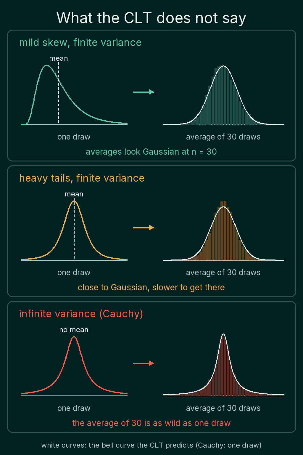
How large $n$ has to be depends on the shape of the data. For mildly skewed data, $n$ around 30 is the usual anchor. For heavily skewed or long-tailed data, it can take thousands.

If the variance is infinite, the theorem does not apply in this form. The Cauchy distribution is a bell-like curve with tails so heavy that it has no mean and no variance. Averaging more draws does not settle it down. Compare five averages of a million draws each, from a standard normal and from a Cauchy:

1import torch
2from torch.distributions import Cauchy, Normal
3 
4torch.manual_seed(0)
5for name, dist in (("normal", Normal(0.0, 1.0)), ("cauchy", Cauchy(0.0, 1.0))):
6    averages = [round(dist.sample((1_000_000,)).mean().item(), 3) for _ in range(5)]
7    print(name, averages)
8# normal [-0.002, -0.001, -0.001, 0.001, 0.001]
9# cauchy [1.086, -0.221, 27.844, -0.48, -2.201]

The normal averages agree to within 0.002. The Cauchy averages jump around, and one of them is 27.8, because a single extreme draw out of the million can drag the whole average. The average of $n$ Cauchy draws has the same distribution as one draw, so collecting more data does not help at all.

Three rows comparing one draw with the average of 30 draws: a mildly skewed distribution whose averages look Gaussian at n = 30, a heavy-tailed distribution with finite variance whose averages are close to Gaussian but slower to get there, and a Cauchy distribution whose average of 30 is as wild as one draw.

Common mistakes

Reading the CLT as "the data is Gaussian". It describes the average, not the individual values. A skewed latency distribution stays skewed no matter how much of it you collect.
Expecting precision to grow linearly with data. Ten times the data shrinks the standard error by a factor of $\sqrt{10} = 3.16$, not 10.
Applying the CLT to samples that are not independent. Near-duplicate rows or one user's many sessions carry less information than their count suggests, and $\sigma/\sqrt{n}$ then makes the error bar too narrow.
Trusting $n = 30$ for long-tailed data. Rare extreme values, like occasional very slow requests, can keep the average far from Gaussian until $n$ is in the thousands.

Expected value and variance covers the $\mu$ and $\sigma^2$ that both theorems are about, and the rule that scaling by $1/n$ divides the variance by $n^2$. Covariance vs correlation explains why variances add only for independent quantities. The Gaussian distribution post covers the bell curve the averages approach, including z-scores. Standard error and confidence intervals build directly on the $\sigma/\sqrt{n}$ result.

QuiddityML teaches the law of large numbers and the central limit theorem as two concepts in the Math track's probability unit, and the exercises on them include completing a running_average function and following the tensor shapes through a simulation of 1,000 samples of 30 draws each.