By Sagi Shaier · 18 October 2026 · 8 min read

MLE vs MAP estimation

How maximum likelihood and maximum a posteriori estimation each pick a parameter from data, why MAP gives a sensible answer where MLE overreacts, and how a prior turns into L2 or L1 regularization, with PyTorch examples.

Maximum likelihood estimation (MLE) picks the parameter value under which the observed data is most probable. Maximum a posteriori estimation (MAP) does the same, but also rewards parameter values that were plausible before the data arrived. The difference shows up when data is scarce, and in deep learning it is the difference between training without and with a weight penalty such as weight decay.

Likelihood

A model with a parameter $\theta$ (theta) assigns a probability $p(x \mid \theta)$ to each data point $x$. The vertical bar reads "given": the probability of $x$ when the parameter is $\theta$. For a coin, $\theta$ is the probability of heads, written $p$. A single flip has probability $p$ if it lands heads and $1 - p$ if it lands tails.

The likelihood $L(\theta)$ is the probability of the whole dataset, viewed as a function of $\theta$. If the data points are independent, it is the product of their individual probabilities:

$$L(\theta)=\prod_{i=1}^{n}p(x_i \mid \theta)$$

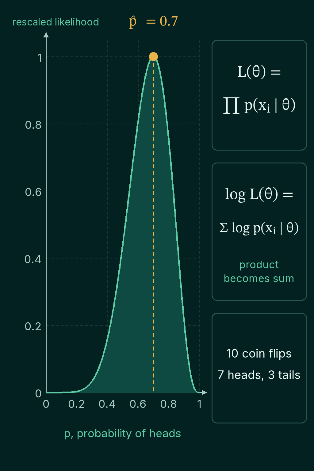
The symbol $\prod$ means "multiply together", in the same way $\sum$ means "add up". Flip a coin 10 times and get 7 heads and 3 tails. The likelihood is $p^7 (1-p)^3$: seven factors of $p$ for the heads, three factors of $1-p$ for the tails. At $p = 0.5$ that is $0.5^{10} = 0.00098$, and at $p = 0.7$ it is $0.7^7 \times 0.3^3 = 0.0022$, more than twice as large.

Maximum likelihood estimation

MLE picks the value of $\theta$ with the largest likelihood:

$$\hat{\theta}_{MLE}=\arg\max_{\theta} L(\theta)$$

$\arg\max$ means "the input that gives the largest output". For 7 heads in 10 flips the answer is $\hat{p} = 0.7$, the observed fraction of heads.

In practice the likelihood is replaced by its logarithm, the log-likelihood, which turns the product into a sum:

$$\log L(\theta)=\sum_{i=1}^{n}\log p(x_i \mid \theta)$$

The log is an increasing function, so the $\theta$ that maximizes $\log L$ is the same one that maximizes $L$. The reason to switch is numerical. A product of many probabilities shrinks toward zero fast, and a computer stores it as exactly zero long before the data runs out:

1import torch
2 
3probs = torch.full((1_000,), 0.5)      # 1,000 points, each with probability 0.5
4print(probs.prod().item())             # the likelihood underflows to zero
5print(round(probs.log().sum().item(), 1))
6# 0.0
7# -693.1

The likelihood of 1,000 data points is too small for a float to hold, while the log-likelihood is an ordinary number. A grid search over candidate values of $p$ finds the coin's MLE from the log-likelihood $7 \log p + 3 \log(1-p)$:

1import torch
2 
3thetas = torch.linspace(0.001, 0.999, 999)    # candidate values of p
4heads, flips = 7, 10
5log_lik = heads * thetas.log() + (flips - heads) * (1 - thetas).log()
6print(round(thetas[log_lik.argmax()].item(), 3))
7# 0.7

argmax() returns the position of the largest value, so thetas[log_lik.argmax()] is the best candidate. The picture shows the same likelihood curve, rescaled so its peak is 1:

The likelihood of 7 heads in 10 coin flips as a function of p, the probability of heads, rescaled so the peak is 1, with the peak marked at p-hat = 0.7, next to the product formula for L of theta and the log-likelihood as a sum of log probabilities.

MLE for a Gaussian

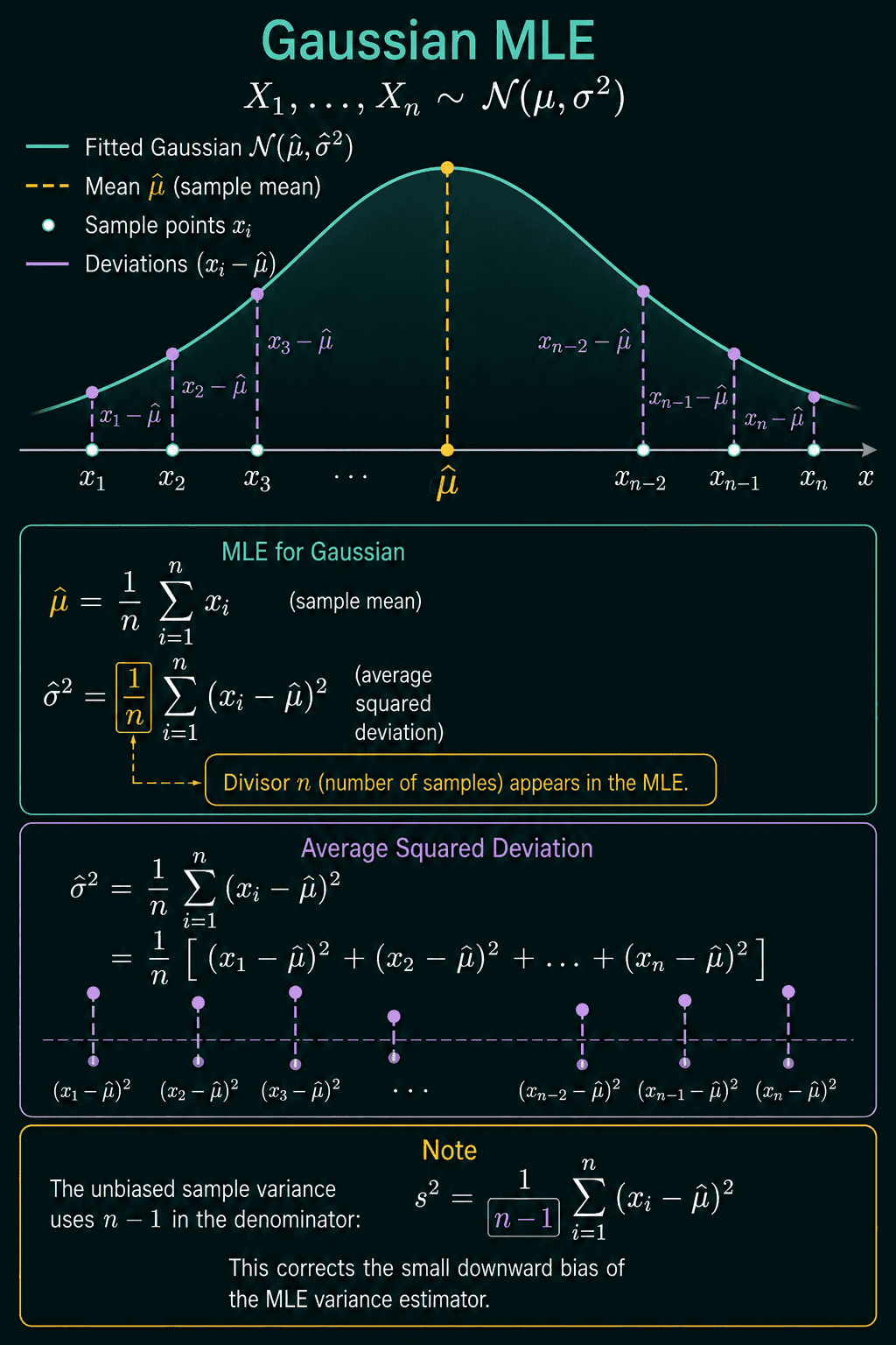
For data from a Gaussian (bell-curve) distribution with mean $\mu$ and variance $\sigma^2$, MLE gives two familiar formulas. The mean estimate is the sample average, and the variance estimate is the average squared distance from it:

$$\hat\mu_{MLE} = \frac{1}{n}\sum_{i=1}^n x_i$$

$$\hat\sigma^2_{MLE} = \frac{1}{n}\sum_{i=1}^n (x_i - \hat\mu)^2$$

The variance divides by $n$, not $n-1$. Take the values 2, 4, 4, 5 and 10. Their mean is 5, and the squared distances from it are 9, 1, 1, 0 and 25, which add up to 36. MLE divides by 5 and gets 7.2. The unbiased sample variance divides by $n - 1 = 4$ and gets 9.0. In PyTorch, x.var(correction=0) divides by $n$ and x.var() divides by $n-1$:

1import torch
2 
3x = torch.tensor([2.0, 4.0, 4.0, 5.0, 10.0])
4mu = x.mean()
5var_mle = ((x - mu) ** 2).mean()        # divides by n
6print(mu.item(), round(var_mle.item(), 2))
7print(round(x.var(correction=0).item(), 2), round(x.var().item(), 2))
8# 5.0 7.2
9# 7.2 9.0

Both are correct answers to different questions. The MLE is the variance that makes the observed data most probable. The $n-1$ version corrects the MLE's tendency to come out a little too small on average, which is what confidence intervals need.

A fitted Gaussian over sample points x1 to xn with the deviations from the sample mean drawn as vertical lines, the MLE formulas for the mean and the variance with the divisor n highlighted, and a note that the unbiased sample variance uses n minus 1.

Common losses are negative log-likelihoods

Training a model by minimizing a loss is often MLE in disguise. Minimizing the negative log-likelihood is the same as maximizing the likelihood, and for common assumptions about the targets it turns into a familiar loss:

If a regression target is the prediction $\hat{y}$ plus Gaussian noise, the negative log-likelihood is squared error, up to a constant and a scale.
If the noise follows a Laplace distribution, a sharper-peaked bell with heavier tails, it is absolute error.
If the target is one of $K$ classes and the model outputs a probability $\hat{y}_k$ for each class $k$, it is cross-entropy, $-\log \hat{y}_k$ for the true class.

In the picture, $\mathrm{Cat}$ is the categorical distribution over the $K$ classes. $1\{y = k\}$ is 1 for the true class and 0 for the others, so only the true class's $\log \hat{y}_k$ survives the sum:

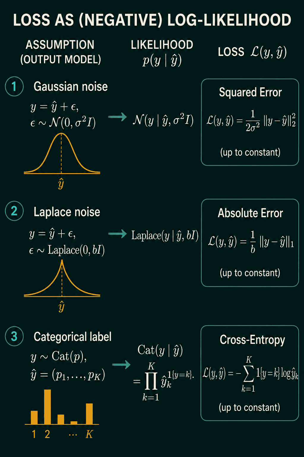
Three rows: Gaussian noise around the prediction gives a Gaussian likelihood and squared error, Laplace noise gives absolute error, and a categorical label gives a product over classes and cross-entropy, each loss up to a constant.

Choosing a loss is also choosing an assumption about how the targets vary around the model's prediction. The maximum likelihood estimation post works through both derivations step by step.

Where MLE overreacts

Flip a coin 3 times and get 3 heads. The MLE is $\hat{p} = 3/3 = 1.0$, a coin that never lands tails. Nothing in the likelihood can argue with that, because the likelihood only knows about those 3 flips. A sensible guess still leaves room for tails on the next flip, because coins are usually close to fair.

That earlier belief can be written as a probability distribution over the parameter, called the prior, $p(\theta)$. Combining it with the likelihood gives the posterior $p(\theta \mid D)$, the distribution of $\theta$ after seeing the data $D$. By Bayes' theorem the posterior is proportional to the likelihood times the prior:

$$p(\theta \mid D) \propto p(D \mid \theta)\,p(\theta)$$

The symbol $\propto$ means "proportional to": equal up to a constant that does not depend on $\theta$, which does not change where the peak is.

Maximum a posteriori estimation

MAP picks the value of $\theta$ at the peak of the posterior. Taking logs turns the product into a sum, as before:

$$\hat{\theta}_{MAP}=\arg\max_{\theta} \left[\log p(D \mid \theta)+\log p(\theta)\right]$$

The first term is the log-likelihood, the same one MLE maximizes. The second term, the log-prior, rewards values of $\theta$ that were plausible before seeing this dataset. MAP is MLE plus one extra term.

For the coin, a prior that favors values near 0.5 is the Beta(2, 2) distribution, whose density is proportional to $p(1-p)$. Its log is $\log p + \log(1-p)$, up to a constant. Score each candidate with log_lik + log_prior and take the best one:

1import torch
2 
3thetas = torch.linspace(0.001, 0.999, 999)
4log_prior = thetas.log() + (1 - thetas).log()       # Beta(2, 2), up to a constant
5 
6for heads, flips in ((3, 3), (30, 30), (300, 300)):
7    log_lik = heads * thetas.log() + (flips - heads) * (1 - thetas).log()
8    mle = torch.tensor(heads / flips)               # MLE in closed form
9    objective = log_lik + log_prior
10    map_ = thetas[objective.argmax()]
11    print(heads, flips, round(mle.item(), 3), round(map_.item(), 3))
12# 3 3 1.0 0.8
13# 30 30 1.0 0.969
14# 300 300 1.0 0.997

After 3 heads in 3 flips, MAP says 0.8 instead of 1.0. After 30 heads in 30 flips it says 0.969, and after 300 it says 0.997. The prior's term stays the same size while the log-likelihood grows with every flip, so with enough data the two estimates come together. MAP can keep an implausible value from winning, unless the data supports it strongly.

How a prior pulls the estimate

The picture shows a parameter $\theta$ with a prior centered at 0 and a likelihood whose peak, the MLE, is at 2. The posterior sits between them, with its peak at 1.34. That peak is the MAP estimate:

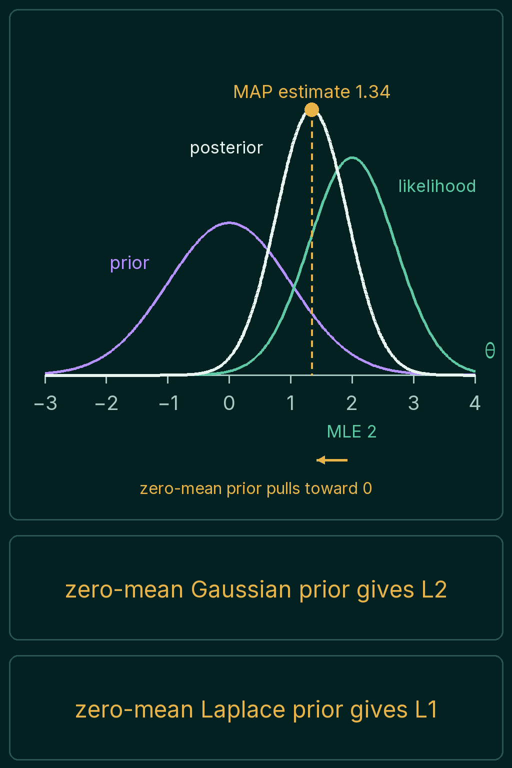
A prior bell curve centered at 0, a likelihood bell curve centered at the MLE of 2, and a narrower posterior curve between them with its peak, the MAP estimate, at 1.34, an arrow showing the zero-mean prior pulling the estimate from 2 toward 0, and two boxes saying a zero-mean Gaussian prior gives L2 and a zero-mean Laplace prior gives L1.

The same grid search reproduces it. Here the likelihood comes from one observation $x = 2$ with Gaussian noise of standard deviation 0.7, and the prior is a Gaussian with mean 0 and standard deviation 1:

1import torch
2from torch.distributions import Normal
3 
4thetas = torch.linspace(-3, 4, 7_001)
5log_lik = Normal(thetas, 0.7).log_prob(torch.tensor(2.0))   # one observation, x = 2
6log_prior = Normal(0.0, 1.0).log_prob(thetas)               # zero-mean prior
7 
8print(round(thetas[log_lik.argmax()].item(), 3))
9print(round(thetas[(log_lik + log_prior).argmax()].item(), 3))
10# 2.0
11# 1.342

The MLE is 2.0, and the prior pulls the MAP estimate back to 1.342.

A prior is a regularizer

Adding a penalty to the loss that discourages extreme parameter values is called regularization. MAP is the probabilistic version of the same idea, because the log-prior is exactly such a penalty.

A Gaussian prior with mean 0 and standard deviation $\tau$ (tau) has log-density $-\theta^2/(2\tau^2)$ plus a constant. For a whole vector of weights $\theta$, maximizing the log-prior is the same as minimizing

$$\frac{1}{2\tau^2}\|\theta\|_2^2$$

where $\|\theta\|_2^2$ is the sum of the squared weights. That is the L2 penalty, which deep learning usually calls weight decay. A smaller $\tau$, a prior more confident that weights are near 0, gives a stronger penalty. A zero-mean Laplace prior with scale $b$ gives

$$\frac{1}{b}\|\theta\|_1$$

the sum of absolute weights, called the L1 penalty.

The zero mean is what makes these penalties pull toward 0. A Gaussian prior centered at some other value $\mu_0$ gives $(1/(2\tau^2))\|\theta - \mu_0\|_2^2$, which pulls the estimate toward $\mu_0$ instead.

Which one to use, and common mistakes

MLE is the default when data is plentiful, and it is what training with a plain loss and no penalty computes. MAP is the better choice when data is scarce or a parameter has a sensible default, and in deep learning that usually means adding weight decay or an L1 penalty to the loss. With a lot of data the two give nearly the same answer, as the 300-flip run shows.

Trusting MLE on a handful of examples. Three flips are enough to make MLE declare a coin that never lands tails.
Forgetting what the penalty assumes. Weight decay is a zero-mean Gaussian prior on the weights, a belief that small weights are more plausible.
Mixing up the variance divisors. The Gaussian MLE divides by $n$, and the unbiased sample variance divides by $n - 1$. x.var() in PyTorch uses $n - 1$ by default.
Multiplying probabilities instead of adding log-probabilities. The product underflows to zero, as it did for 1,000 points above.

The maximum likelihood estimation post derives mean squared error and cross-entropy from MLE in full. Bayes' theorem explains the posterior-equals-likelihood-times-prior step. The common probability distributions post covers the Beta distribution used as the coin's prior. Regularization and weight decay vs L2 regularization cover the penalties a prior turns into, from the training side.

QuiddityML teaches maximum likelihood and maximum a posteriori estimation as two concepts in the Math track's probability unit, and the exercises on them include filling in the Gaussian MLE formulas and implementing map_estimate, which picks the best of a set of candidate values.